From Word2Vec to BERT: The Evolution of Language Embeddings

August 26, 2025 · #llm

If you’ve prompted Llama to write a Python script, watched GitHub Copilot complete a tricky function, or just typed a “near human” query into Google, you’ve seen the output. It feels like magic. But as engineers, we know the truth: it’s not magic, it’s just a stack of brilliant, hard-won abstractions.

Underpinning all this modern wizardry is one fundamental capability: teaching a machine that only knows FLOATs and INTs to understand the subtle, context-rich, and ambiguous human language. How do you quantify the difference between “bank” (a place for money) and “bank” (the side of a river)? How do you represent “king” and “queen” as being closer to each other than to “avocado”?

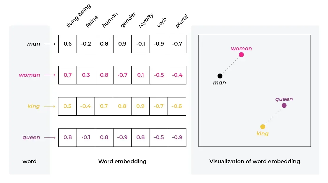
The answer is language embeddings, vector representations of text that encode meaning as points in a high-dimensional space. And the story of how we got from the first clunky attempts to the powerful models of today isn’t a neat, linear progression. It’s a classic engineering tale of bottlenecks, clever hacks, and paradigm shifts that solved one problem only to reveal the next, more complex one.

This isn’t just another academic overview. We’re going to walk the path from an engineer’s perspective. We’ll start with the breakthrough that gave us our first real semantic tool, Word2Vec, and follow the trail of innovations that led to BERT, the model that truly unlocked our current era of NLP. Let’s get under the hood.

On the dead end of One-Hot Encoding

Alright, first principles. Before we can do any fancy math, we have to solve a basic data representation problem. Our machine speaks in numbers, and we have a vocabulary of words. The most straightforward approach, the one you’d probably code up in an hour if asked, is to build an index.

Let’s say our entire vocabulary is ["king", "queen", "man", "woman"]. We can map them to IDs:

• king: 0

• queen: 1

• man: 2

• woman: 3

Simple enough. To make this a vector, we can just turn that index into a “hot” signal in a vector of zeros. This is One-Hot Encoding.

• king = [1, 0, 0, 0]

• queen = [0, 1, 0, 0]

• man = [0, 0, 1, 0]

• woman = [0, 0, 0, 1]

This works. It’s unambiguous. But there are challenges:

1. The Scalability Nightmare

Our toy vocabulary has 4 words, so our vectors are 4-dimensional. A production-level vocabulary for English has at least 50,000 words. So, the dimensionality of your vectors (d) becomes equal to the size of your vocabulary (|V|).

d = |V| ≈ 50,000

Every single word is now a 50,000-dimensional vector that is almost entirely zeros. Storing and performing matrix multiplications on these monstrously sparse vectors is computationally brutal and memory-inefficient. It just doesn’t scale.

2. The Meaningless Vector Problem

This is the killer. For these vectors to be useful, they need to encode meaning. A good way to measure the relationship between two vectors is to calculate the cosine similarity, which is closely related to their dot product. Let’s see what happens.

What’s the relationship between “king” and “queen”?

dot([1,0,0,0], [0,1,0,0]) = 0

What’s the relationship between “king” and “man”?

dot([1,0,0,0], [0,0,1,0]) = 0

Every vector is perfectly orthogonal to every other vector. The mathematical similarity between king and queen is exactly the same as the similarity between king and screwdriver. The system knows the words are different, but it has zero concept of how they relate.

This was the wall we were up against. We had a way to represent words as unique identifiers, but not as concepts. We needed vectors that were not just addresses, but actual coordinates in a “map of meaning.”

The Leap to Meaning: Word2Vec and The Geometric “Aha!” Moment

So, one-hot vectors were a dead end. They were sparse (means the vector had too many zero - which means no signal), scaled poorly, and were semantically useless. The field needed a way to bake meaning directly into the vector itself.

The revolution came in 2013 from a team at Google with a paper that introduced Word2Vec. The model was built on a simple but profound linguistic idea, famously summarized by linguist J.R. Firth: “You shall know a word by the company it keeps.”

Instead of assigning words to arbitrary, orthogonal slots, the Word2Vec model learns representations by predicting context. The training process is a brilliant hack. You take a massive corpus of text (like all of Wikipedia), slide a window across it, and train a shallow neural network to do one of two simple things:

1. Skip-gram: Given a target word (e.g., “king”), predict its surrounding context words (e.g., “queen,” “throne,” “kingdom”).

2. Continuous Bag of Words (CBOW): Given the context words, predict the target word.

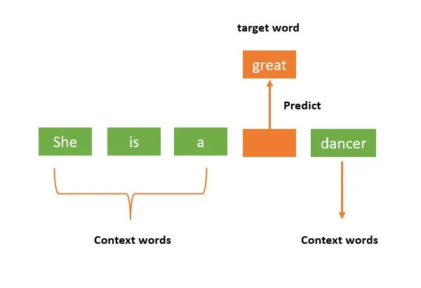
The prediction task itself isn’t the point. The magic is in the side effect. As the network gets better at this game, its internal weights evolve. These weights are, in fact, the embeddings. You train the model, let it converge, and then you throw away the network and just keep the learned weight matrix.

What came out was astounding.

Instead of 50,000-dimensional sparse vectors, we now had dense, 300-dimensional vectors. And these vectors weren’t just random points; they organized themselves into a “thought space” where the geometry mapped to semantics. This led to the legendary example that defined the era:

vector('king') - vector('man') + vector('woman')

When you performed this arithmetic, the resulting vector was closer to vector('queen') than any other word in the vocabulary.

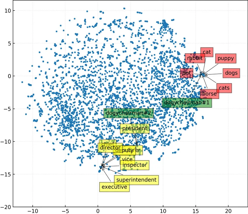
This was the “Aha!” moment. These static embeddings, along with contemporaries like GloVe from Stanford, became the bedrock of NLP for years. We could finally compute a meaningful similarity between words.

But engineering is a relentless process of finding the next bottleneck. And these static embeddings had a huge one. The word “bank” had one and only one vector.

Consider these two sentences:

1. “I deposited my money at the bank.”

2. “The boat was moored on the river bank.”

Word2Vec would produce the exact same vector for “bank” in both cases.

For machines to truly understand language, they couldn’t just have a dictionary. They needed to be able to read a sentence and figure out which definition to use. This was the next wall we had to break through.

The Contextual Age: LSTMs and the Burden of Sequential Thought

The “bank” problem was a clear and present danger to our goal of true language understanding. We had vectors that understood “what a word is in general” but not “what this word means right now.” The solution was conceptually simple: to understand a word’s specific meaning, the model needed to read the entire sentence it appeared in.

The go-to architecture for this kind of sequential data was the Recurrent Neural Network (RNN). An RNN is effectively a loop. For each word in a sentence, it performs a calculation, updates an internal “memory” or hidden state, and then carries that state forward to the next word. Think of it like a single-threaded processor executing a program line by line, maintaining its state in registers as it goes.

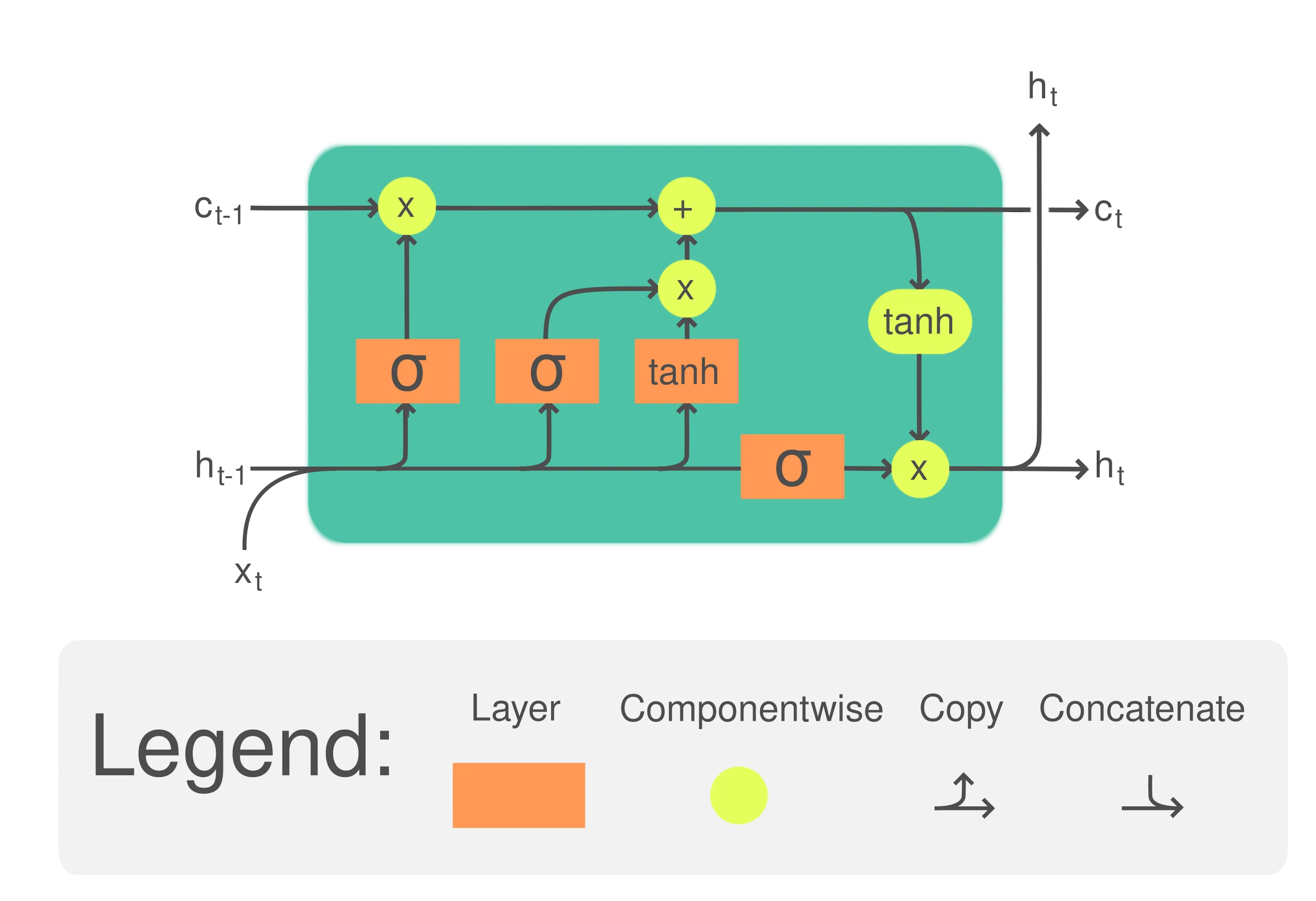
A more robust and popular variant was the Long Short-Term Memory (LSTM) network. LSTMs were a sophisticated type of RNN with internal “gates” that allowed them to make more intelligent decisions about what information to remember and what to forget from their hidden state. This made them better at handling longer sentences where early context might be important later on.

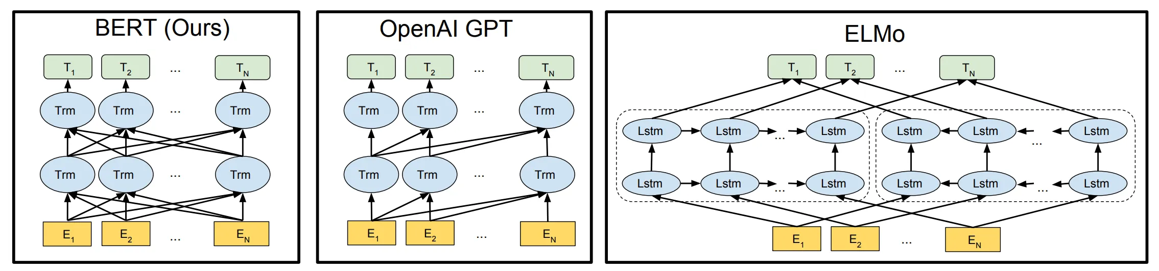
This approach culminated in models like ELMo (Embeddings from Language Models), released in early 2018. ELMo was clever. It processed a sentence with two powerful, independent LSTMs: one reading from left-to-right, and another reading from right-to-left. It then concatenated the hidden states from both LSTMs.

For the first time, we had a popular and effective model that produced truly contextual embeddings. The vector for “bank” in “river bank” was now genuinely different from the vector for “bank” in “investment bank,” because its representation was a function of the entire sequence around it. Problem solved, right?

Not quite. From a systems and hardware perspective, this sequential approach came with a heavy price.

The core operation of an LSTM looks something like this:

The hidden state at the current timestep t is a function of the current input ht-1 and the hidden state from the previous timestep ht-1. This is an inherently sequential dependency. You cannot calculate step 5 until you have finished calculating step 4.

This serial nature is a massive bottleneck that fights tooth-and-nail against modern hardware. We have GPUs with thousands of cores designed for massively parallel computation, yet we were forcing our models to think one word at a time.

We had achieved context, but at the cost of parallelism and perfect memory.

The Paradigm Shift: “Attention Is All You Need”

The slowness of sequential models was a known, accepted pain point. We had context, but we were paying a heavy performance tax for it. Then, in mid-2017, a paper from Google researchers landed with a title that was both incredibly bold and, in hindsight, 100% correct: “Attention Is All You Need.”

This paper introduced the Transformer, an architecture that completely threw out the old playbook of recurrence. No more loops. No more sequential processing. No more ht = f(ht-1, ht-1).

The core idea was a mechanism called self-attention.

Instead of processing a sentence one word at a time, the Transformer digests it all at once. For each word, the self-attention mechanism allows it to look at every other word in the sentence simultaneously and ask a simple question: “How relevant is each of these other words to my own meaning in this specific context?”

This architectural leap unlocked two earth-shattering benefits that LSTMs could never offer.

1. Massive Parallelism. This was the holy grail. This meant we could train vastly larger models on vastly larger datasets, orders of magnitude faster than the old RNN/LSTM regime. It was a perfect marriage of algorithm and hardware.

2. O(1) Path Length. In an LSTM, for information to travel from the first word of a paragraph to the last, it had to pass sequentially through every single intermediate step, with the risk of getting distorted or forgotten along the way. In a Transformer, the path length between any two words in the sequence is O(1).

Now, all we needed was the right fuel and the right training strategy to turn this powerful engine into the apex predator of NLP.

The Apex Predator: BERT and the Power of Bidirectionality

The Transformer gave us a revolutionary engine. Now, the question was how to train it for maximum effect. For years, the standard approach for language models (like the early GPTs) was “auto-regressive” pre-training: read a sequence of words and predict the next one. This is essentially a very powerful autocomplete. It’s useful, but inherently one-directional (left-to-right). To achieve a deep understanding of context, you need to look both ways.

In late 2018, another team at Google released the model that put it all together: BERT (Bidirectional Encoder Representations from Transformers). BERT took the Transformer architecture and combined it with a brilliant new pre-training strategy that forced the model to learn context from both directions simultaneously.

BERT wasn’t trained to predict the next word. Instead, it was given two ingenious tasks designed to build a much deeper, more robust understanding of language.

1. Masked Language Model (MLM): The “Fill in the Blank” Hack

This was the genius at the heart of BERT. Instead of showing the model a complete sentence, the researchers randomly hid about 15% of the words, replacing them with a special [MASK] token. The model’s only job was to predict the original words that belonged in the masks.

Consider the sentence:
My dog is a Golden [MASK] and he loves to [MASK] in the lake.

This simple “fill in the blank” game forced the model to develop a deep, bidirectional understanding of how words fit together. It moved from being a simple predictor to a true context understander.

2. Next Sentence Prediction (NSP)

To capture relationships between entire sentences, BERT was also trained on a second task. The model was given two sentences, A and B, and had to predict whether sentence B was the actual sentence that followed A in the original text or just a random sentence from the corpus. This taught the model a sense of narrative flow and logical coherence between chunks of text.

The result was a game-changer. BERT wasn’t just another model you trained from scratch. It was a pre-trained foundational artifact. Google had done the massively expensive part: training it on a gargantuan amount of text (the entire English Wikipedia and a huge book corpus).

You could then download this pre-trained BERT and “fine-tune” it on your specific task (like sentiment analysis or spam detection) with a relatively tiny amount of data and compute. It obliterated nearly every NLP benchmark and leaderboard. The era of BERT had begun, and “fine-tuning a pre-trained Transformer” became the new default for virtually any NLP problem.

Conclusion: From Static Points to Dynamic Vectors

The journey from Word2Vec to BERT isn’t just a timeline of academic papers; it’s a classic engineering story. It’s a narrative of identifying a bottleneck, deploying a clever hack to solve it, and in doing so, revealing the next, deeper problem in the stack.

We started with a revolutionary idea: that meaning could be mapped geometrically. Word2Vec gave us static points in a thought-space, a huge leap from meaningless one-hot vectors, but failed at the first sign of ambiguity.

We patched that bug with LSTMs, creating sequential models like ELMo that could finally understand context. But we paid a heavy price in performance, forcing our massively parallel GPUs to think in a slow, single-threaded way.

The Transformer architecture shattered that bottleneck. By introducing self-attention, it untethered us from sequential processing and married our algorithms to our hardware. BERT then provided the masterstroke training strategy, the masked language model, that fully utilized this new architecture, forcing models to learn a deep, bidirectional understanding of language.

This final architectural leap, from static to dynamic, from sequential to parallel, is the foundation upon which everything we see today is built. The powerful generative models like the GPT series, Google’s T5 family, and yes, Meta’s own Llama, all stand on the shoulders of the Transformer architecture that BERT proved so decisively.

And this concludes our journey in understanding language embeddings.