From Brute Force to Finesse: The Story of Parameter-Efficient Fine-Tuning (PEFT)

August 19, 2025 · #llm

Last week I was in AI4 conference that had the highest concentration of C-suit and directors. All of them were talking about different aspect of how to make these models really work. Some where talking about RAG, some others about fine tuning and many about what ever they do, models don’t work really. Well, I found it fascinating that what we, as individual users, think as state of the art intelligence; corporate users find non-usable.

They talked about horror stories of fine tuning a 70B parameter model and how just the cost of storing multiple 140GB snapshot of those models were sinking the ship, let alone the cost of compute to fine tune them.

The unfortunate fact is that with wrong data and recipe, fully fine tuning a model actually makes it dumber rather than smarter. Reasoning capabilities degrades with each additional step.

And in the crowd, some where talking about PEFT as a better way of fine tuning the model. It’s about the shift from brute-force updates to surgical fine-tuning. In this article, we talk about how it works.

Alright, So What’s the First Fix? The Adapter.

So, full fine-tuning is a dumpster fire. We’ve established that. It’s a resource hog, it creates massive artifacts, and it breaks the model as often as it helps.

The first serious attempt to get around this came out of the BERT era, around 2019. The paper from Houlsby et al. was a real “aha!” moment. The core idea was simple, almost like a systems design pattern: instead of modifying the core service (the frozen LLM), let’s inject some middleware.

They called them Adapter Modules.

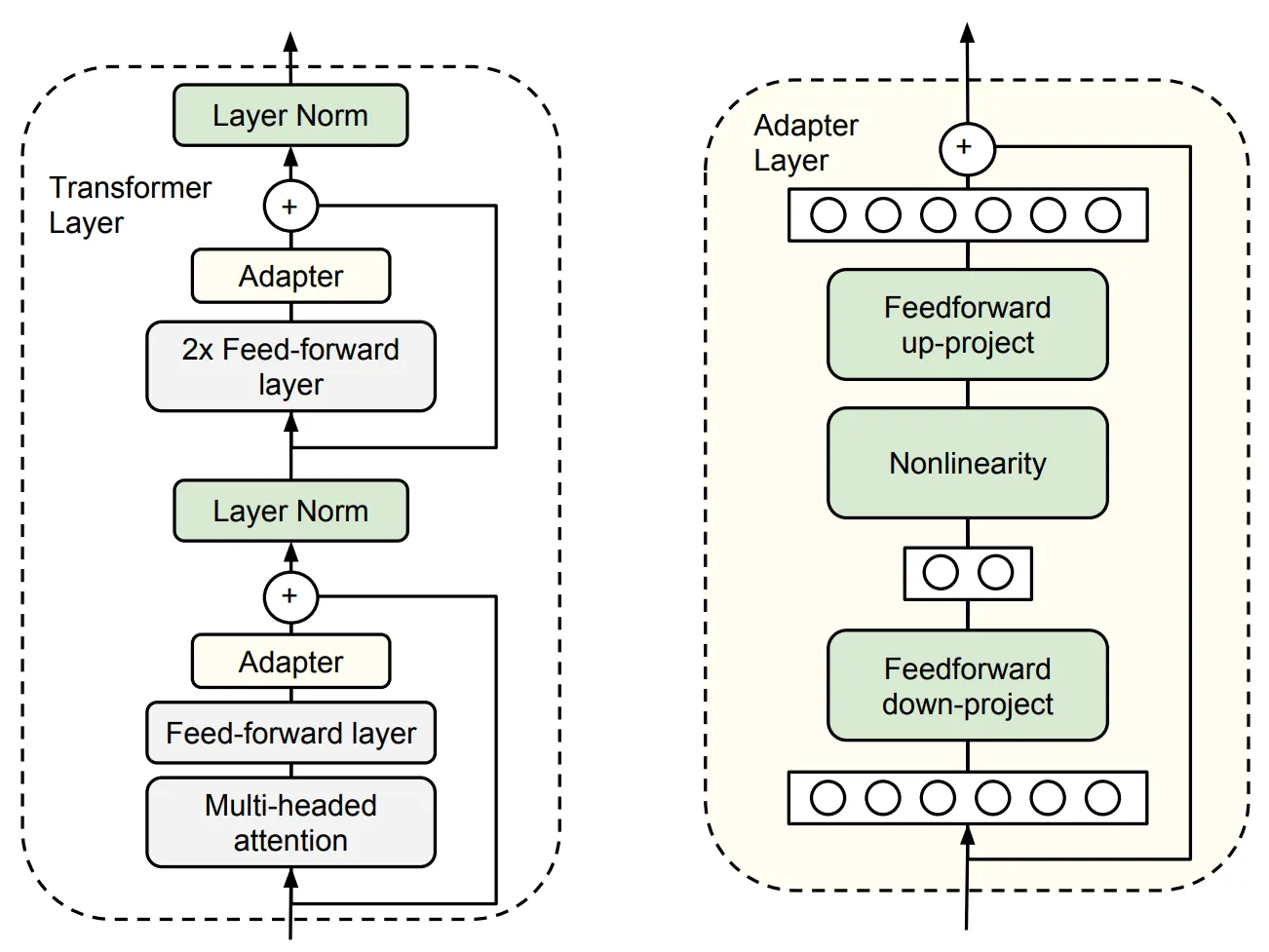
The concept is dead simple. You take your big, frozen, pre-trained transformer block. Inside it, you bolt on two tiny, trainable feed-forward layers. It’s a classic bottleneck architecture:

1. A linear layer projects the huge hidden state (e.g., 4096 dimensions) down to a tiny, manageable dimension (e.g., 64).

2. A non-linearity (like ReLU) gets applied.

3. Another linear layer projects it back up to the original 4096 dimensions.

That’s it. During training, you freeze everything else. The multi-billion parameter model doesn’t see a single gradient update. Only these tiny bottleneck layers, maybe a few hundred thousand parameters in total, are being trained.

The result? You get task-specific behavior, but your checkpoint is just the weights for these tiny adapters, not another 140GB model. It was a huge step forward. You could now have one base model and a directory of small adapter files for different tasks.

But it wasn’t a silver bullet. It came with a critical engineering trade-off: inference latency.

Because these adapters are new layers inside the model, you’re adding operations to every single forward pass. For every token you generate, you’re paying a new “adapter tax.”

So, while adapters proved the core thesis—that you could specialize a model with a tiny parameter delta—the latency cost meant the search for a truly efficient, zero-overhead solution wasn’t over. We needed a way to get the same benefit without adding new ops to the critical path.

The Real Breakthrough: LoRA Solves the Latency Problem

Okay, so Adapters were clever. They proved you could get specialization with a small parameter delta. But the inference latency tax was a deal-breaker for a lot of real-world services. The engineering requirement was clear: we need the parameter efficiency of adapters, but with the zero-overhead performance of a fully fine-tuned model.

This is where LoRA (Low-Rank Adaptation) came in and changed the game. The paper from Microsoft researchers in 2021 wasn’t just another tweak; it was a fundamentally different approach based on a slick linear algebra insight.

The core idea is this: When we fine-tune a model, the update to the weights (let’s call it ΔW) doesn’t have to be a giant, full-rank matrix. The hypothesis is that the “change” needed for a new task has a low “intrinsic rank.” In plain English, the massive change matrix can be effectively compressed or approximated by multiplying two much, much smaller matrices.

Here’s the breakdown, skipping the academic Greek letters for a second.

A standard weight update looks like this:

Here, W0 is the original frozen weight matrix, and ΔW is the change we learn. In full fine-tuning, ΔW is the same massive size as W0.

LoRA’s core hack is to say we can approximate that giant ΔW like this:

Where A and B are our new, trainable matrices. A is tall and skinny, and B is short and fat. For a weight matrix of 4096x4096, A might be 4096x8 and B would be 8x4096. The number 8 here is the rank (r), and it’s a hyperparameter we can tune.

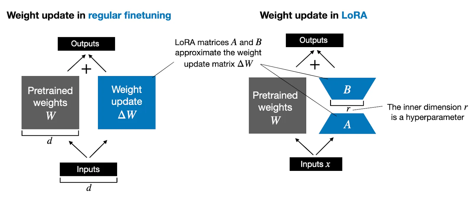
So instead of training the 16.7 million parameters in W, we’re only training the (4096 * 8) + (8 * 4096) = 65,536 parameters in A and B. That’s a ~99.6% reduction in trainable parameters for that single layer.

But here’s the killer feature, the one that solves the adapter problem.

During training, we keep W0 frozen and just update A and B. But for deployment, we can do a one-time, offline calculation:

This gives us a single, new weight matrix, Wmerged. We then deploy the model with this merged matrix. The model’s architecture is now identical to the original. There are no extra layers, no new operations, no adapter tax.

This was the magic bullet. LoRA gave us the best of both worlds:

1. Tiny, portable checkpoints (just the A and B weights).

2. Massively reduced trainable parameters, lowering the VRAM requirements for training.

3. Zero additional latency at inference time after merging.

This is why LoRA became the de-facto standard for PEFT. It addressed the single biggest operational blocker that adapters introduced, making efficient fine-tuning not just possible, but practical for production.

70B on a 4090: The QLoRA Revolution

LoRA fixed the latency issue, and that was huge. But there was still a giant, immovable object in the way of true accessibility: the base model’s memory footprint.

Let’s be blunt. A 70B parameter model, loaded in standard 16-bit precision (fp16), requires 140GB of VRAM. An 80GB A100 can’t even load it, let alone train it. This meant that even with LoRA, fine-tuning was still a multi-GPU, cloud-only affair—complex, expensive, and slow to iterate on. You couldn’t just spin up an experiment on your local machine.

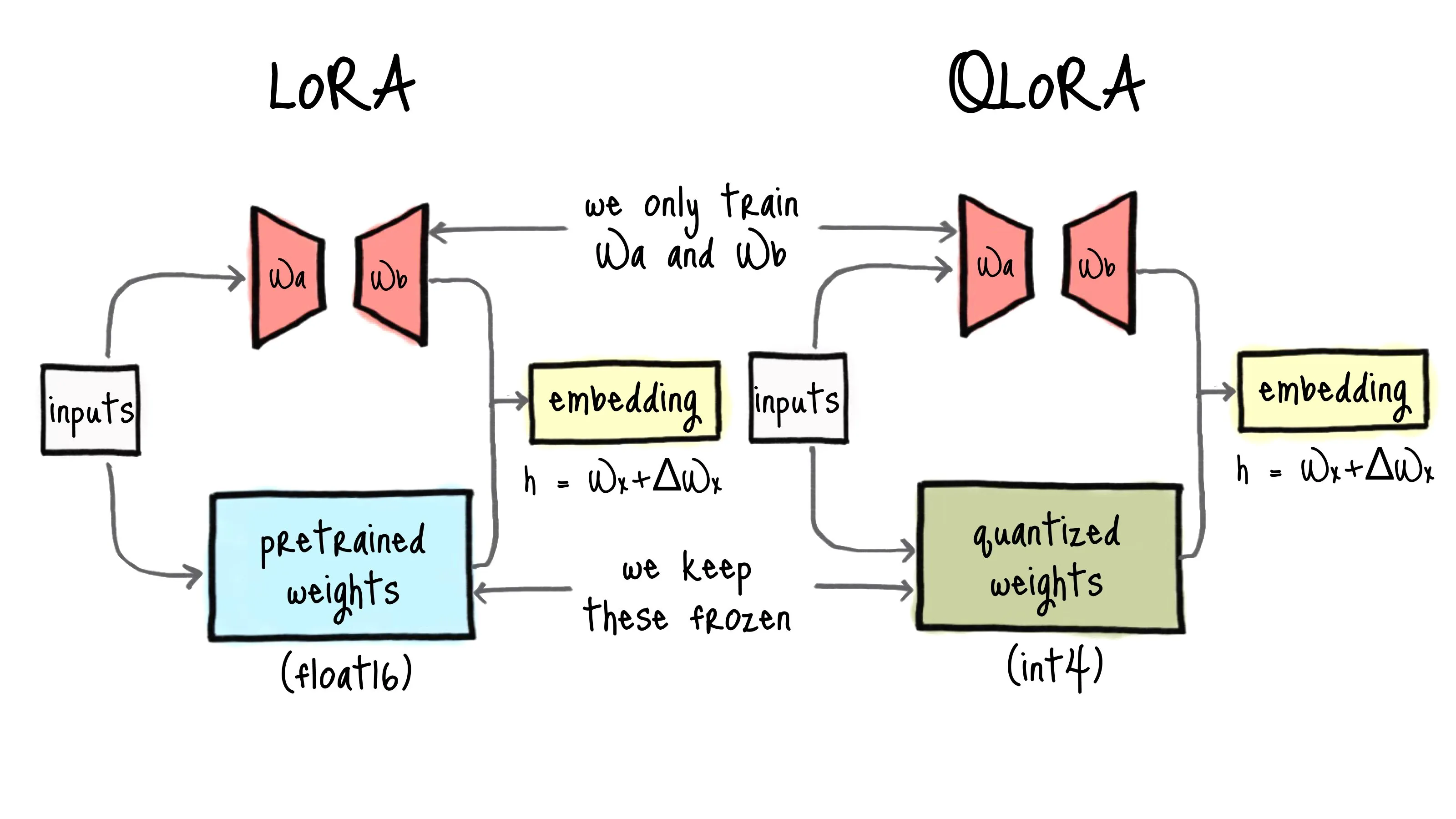
The obvious answer was quantization—using fewer bits to store the model’s weights. People had been doing this for years, typically moving from 16-bit to 8-bit integers (int8 or FP8 for some GPUs that supported it). But it always came with a nasty trade-off: you saved memory, but the model’s performance tanked. The precision loss was just too damaging.

Then, in mid-2023, Tim Dettmers and his team dropped the QLoRA paper, and it was the final piece of the puzzle. QLoRA isn’t just “quantization + LoRA.” It’s a specific, highly-engineered set of techniques that makes aggressive quantization work without the performance hit.

Here’s the technical stack that makes it possible:

1. 4-bit NormalFloat (NF4): This is the core innovation. Instead of a standard 4-bit integer, they designed a new 4-bit float data type that is “information-theoretically optimal” for data that follows a normal distribution—which model weights do. In simple terms, every single one of the 16 possible values in this 4-bit type is assigned to perfectly map the expected bell curve of the weights. This preserves way more information than a naive 4-bit quantization scheme.

2. Double Quantization: This is a clever optimization on top. The quantization process itself requires saving some metadata (quantization constants). Double Quantization reduces the memory footprint of this metadata by quantizing the constants themselves. It’s a second layer of compression that saves an extra ~0.5 bits per parameter.

3. Paged Optimizers: For anyone who has ever battled a CUDA: out of memory error, this is a godsend. It uses the NVIDIA unified memory feature to page optimizer states between GPU and CPU RAM. If you run out of VRAM during a sudden spike (e.g., processing a batch with long sequences), it transparently offloads to system RAM instead of crashing. This makes training far more stable and robust.

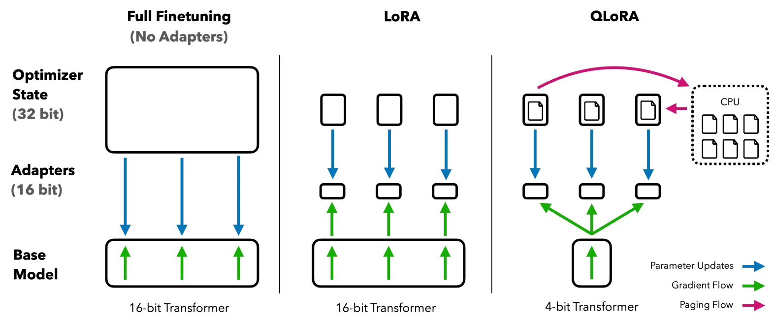
You can load a 70B parameter model, fine-tune it with LoRA, and have it all fit on a single 24GB GPU**.** Suddenly, SOTA fine-tuning was possible on an RTX 4090.

This wasn’t just an incremental improvement; it was a phase change. It democratized the ability to work with these massive models.

Conclusion: A Saner Primitive for Building with AI

Let’s circle back to that AI conference. The room was full of leaders facing a wall. The promise of LLMs was clear, but the engineering reality was a mess of monolithic artifacts, catastrophic forgetting, and spiraling costs. Full fine-tuning wasn’t just expensive; it was an unproductive development loop. It was the wrong primitive for the job.

The journey from Adapters to LoRA and finally to QLoRA wasn’t just a series of incremental improvements. It was a fundamental refactoring of how we interact with these models.

• We went from forking the monolith to shipping a patch.

• We killed the inference latency tax by making the patch mergeable.

• We solved the VRAM wall with a smarter, information-theoretically sound quantization scheme.

What we’re left with is a new, sane development primitive. The ability to fine-tune a 70B model on a single GPU and ship the result as a ~200MB artifact isn’t a neat party trick—it’s the new baseline.

This is a move from monolithic AI development to a modular, composable architecture. We’ve stopped treating these models as fragile, unchangeable black boxes and started engineering them with the precision they deserve.

At its core, the PEFT stack is about finding the path of least resistance. Instead of blindly updating billions of parameters, we’re finding the low-rank pathway—the sparse diff—that represents new knowledge. It’s a more elegant, efficient, and ultimately, more buildable approach. It’s the engineering finesse that finally makes the brute-force power of these titans practical.