Attention Isn't All You Need. You Also Need a Memory Budget

September 2, 2025 · #llm

So you’ve fine-tuned the latest Llama model. The evaluation metrics are stellar, and you’re ready to deploy it. You spin up your inference server, start feeding it concurrent requests with a decent 8k context window, and suddenly you see it: your GPU memory usage skyrockets, your batch size is limited, and your latency per token is nowhere near what you’d hoped. What’s going on?

Your first instinct might be to blame the sheer parameter count of the model—all those billions of weights and the corresponding matrix multiplications. And while those are certainly expensive, they are not the silent killer of inference throughput. The real culprit is a less-famous but far more insidious bottleneck for large context and high-throughput scenarios: the KV Cache.

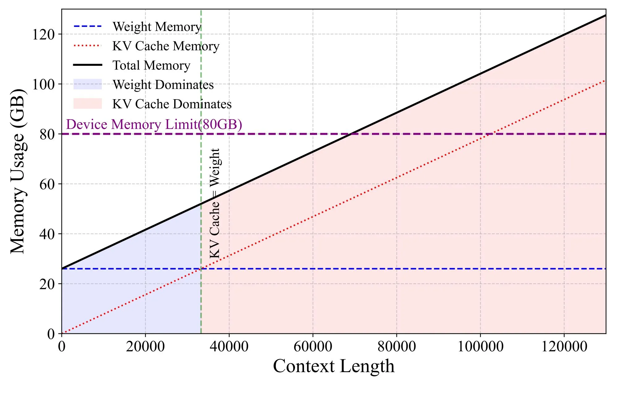
This cache, a clever optimization originally designed to speed up generation, paradoxically becomes one of the biggest memory hogs in any modern LLM.

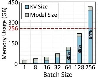
In this post, we’re going to dive deep into the engineering hacks that make today’s powerful models practical. We’ll explore the architectural trade-offs that took us from Multi-Head to Grouped-Query Attention (GQA), and then go down to the metal with the systems-level magic of FlashAttention and its sequels. This is the story of how we started fixing the biggest problem in the “Attention Is All You Need” paradigm.

Vanilla Multi-Head Attention and the KV Cache Beast

To understand the problem, we have to start with the source: the standard Multi-Head Attention (MHA) mechanism from the original “Attention Is All You Need” paper.

The idea was to allow the model to focus on different parts of the input sequence simultaneously. Instead of having one big attention calculation, MHA splits the model’s dimension (d_model) across multiple independent “heads.” Each head gets its own set of learned projection matrices for Query (Q), Key (K), and Value (V). For a model like Llama 2 7B, we have 32 heads, each looking at a different subspace of the embeddings.

This works beautifully for understanding a static piece of text. But things get complicated when we start generating text one token at a time, which is the core task of a decoder-style LLM.

Generating the 501st word in a sequence requires the model to pay attention to the first 500 words. When we then generate the 502nd word, it needs to attend to the first 501 words. Recomputing the Key (K) and Value (V) vectors for all preceding tokens at every single step would be computationally disastrous.

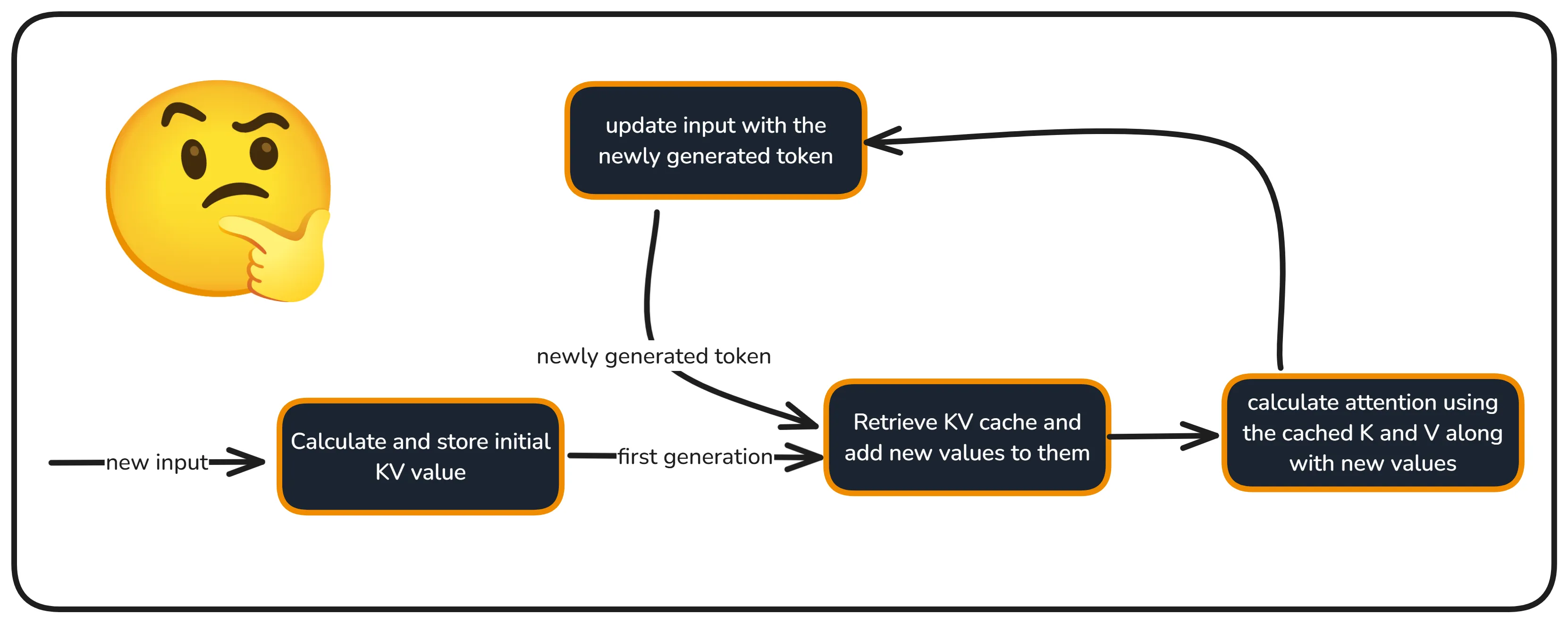
The obvious optimization is to cache them. This is the KV Cache. After each step, we store the K and V vectors we just computed and reuse them in the next step. So, at step T+1, we only need to compute the Q, K, and V for the newest token and append its K and V to our growing cache.

This works. It saves a ton of redundant computation. But in solving one problem, it creates another massive one: memory. The cache grows linearly with the sequence length and the batch size, and the numbers get scary, fast.

Let’s calculate the size of this cache for a single layer:

(The ‘2’ is because we store both K and V vectors.)

Now let’s plug in some real numbers for a single sequence running on a Llama 2 7B model with a standard 8192-token context window:

• batch_size = 1

• sequence_length = 8192 tokens

• d_model = 4096

• precision = 2 bytes (for bfloat16)

That’s 134 megabytes for a single layer. The Llama 2 7B model has 32 layers.

We are burning over 4 gigabytes of premium GPU HBM(High Bandwidth Memory) just to store the state for a single user’s request. The model’s actual weights are ~14 GB. The KV cache is a significant fraction of the total memory footprint.

And what happens when we try to serve a batch of 16 users to maximize throughput?

That’s 69 gigabytes. This much memory is needed just for the temporary state of one forward pass, exceeding the capacity of even high-end GPUs like an A100 (40/80GB) or an H100 (80GB).

This is the KV Cache beast. It’s the single biggest factor limiting the context length and batch size of LLM inference. The model’s weights are static, but this dynamic cache can explode, and taming it became the next great engineering challenge.

(Hope you’re enjoying reading this so far as I’m enjoying writing it! 😍_)_

Multi-Query Attention (MQA) - Brutal but Effective

Faced with a memory bottleneck that grows linearly with the number of attention heads (n_heads), the engineering solution was both radical and brutally direct: What if we just got rid of most of the heads? This is the core idea behind Multi-Query Attention (MQA).

The insight was that the massive KV cache is a direct result of each of the 32 (in Llama’s case) attention heads maintaining its own independent Key and Value projections. But what if they didn’t have to? In MQA, we still keep all the multiple Query heads—allowing the model to “ask” many different questions about the context—but we force them all to share a single Key and Value head.

Instead of each head getting its own perspective of the past, they all have to work with the same, shared representation of the context.

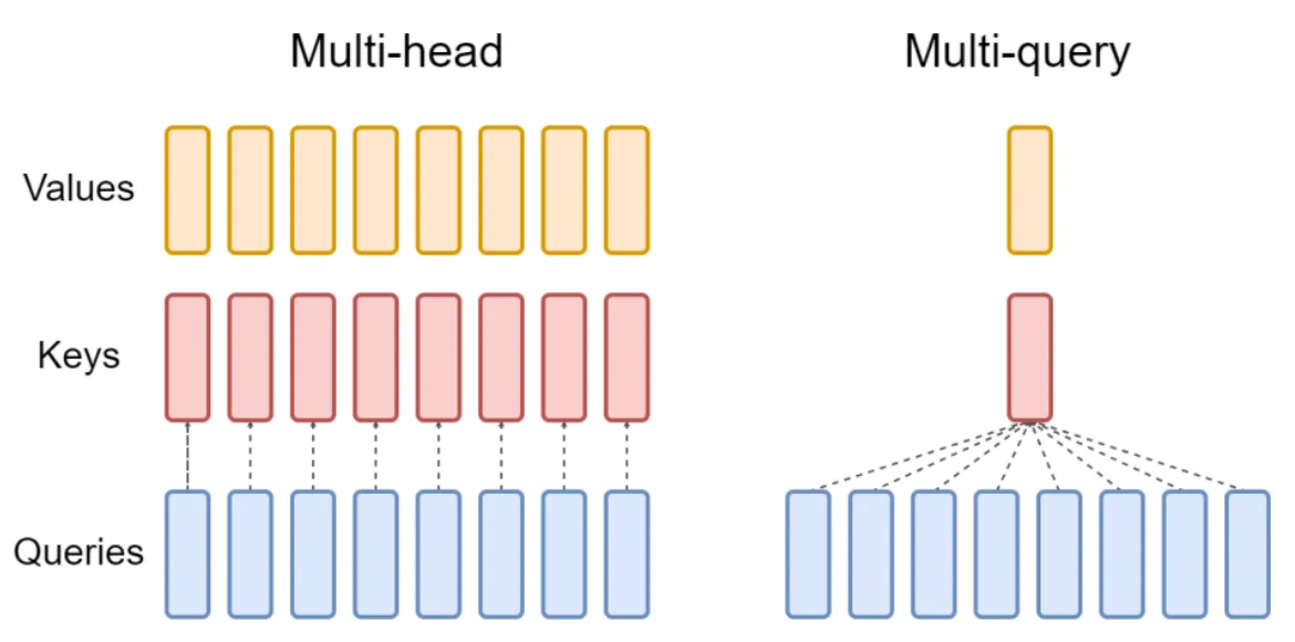
The impact on the KV Cache is exactly what you’d hope for. The cache size is reduced by a factor equal to the number of heads. Let’s revisit our Llama 2 7B example, which has 32 heads:

Vanilla Multi-Head Attention (MHA) Cache Size (per sequence):

Multi-Query Attention (MQA) Cache Size (per sequence):

Since d_head = d_model / n_heads = 4096 / 32 = 128:

The cache size collapses from 4.3 GB to just 134 MB.

This is a monumental reduction. Suddenly, you can fit much larger batches into GPU memory, dramatically increasing server throughput. You can also handle much longer context sequences without memory becoming the immediate bottleneck. It’s a huge win for inference performance.

However, this performance doesn’t come for free. This is a hard architectural trade-off. By forcing all query heads to share a single K and V representation, you create a representational bottleneck. The model might lose some of its nuanced ability to look at the past from different perspectives. The original MHA design allowed one head to focus on syntactic relationships while another focused on semantic ones. MQA forces them all to pull from the same well of information.

The result is often a measurable drop in model quality and perplexity. While some models were designed with MQA from the start (like Google’s PaLM), for many architectures, the quality degradation was too high a price to pay.

Grouped-Query Attention (GQA), The Production Standard

The trade-off was clear: Multi-Head Attention (MHA) offered maximum model quality at a prohibitive memory cost, while Multi-Query Attention (MQA) offered maximum memory savings at a potential quality cost. As is often the case in engineering, the optimal solution wasn’t at either extreme, but in a carefully chosen middle ground: Grouped-Query Attention (GQA).

The idea is an elegant compromise between its two predecessors. Instead of having all Query heads share one Key/Value head (MQA), or giving each Query head its own (MHA), GQA buckets the Query heads into several smaller groups. Each group of Query heads then shares a single Key/Value head.

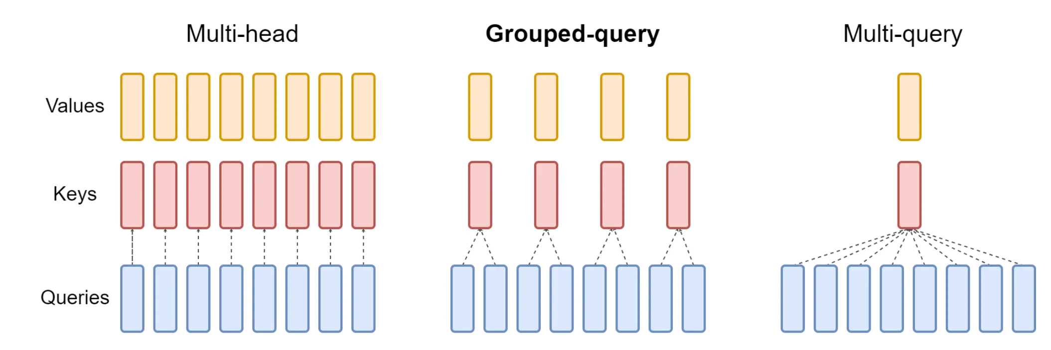
Let’s define N as the total number of Query heads and G as the number of groups (and thus the number of K/V heads).

• In MHA, you have N Query heads and N K/V heads. (G = N)

• In MQA, you have N Query heads and 1 K/V head. (G = 1)

• In GQA, you have N Query heads and G K/V heads, where 1 < G < N.

This isn’t just a theoretical curiosity; this is the production standard used in today’s most powerful open models. Both Llama 2 and Llama 3 are built with Grouped-Query Attention. It is the key architectural feature that allows these models to handle long context windows efficiently while maintaining their state-of-the-art performance.

Let’s look at the numbers for a Llama 2 7B model, which uses 4 groups:

GQA Cache Size (per sequence, G=4):

Or more simply, the MHA cache size divided by the number of groups:
4.3 GB / 8 = ~550 MB

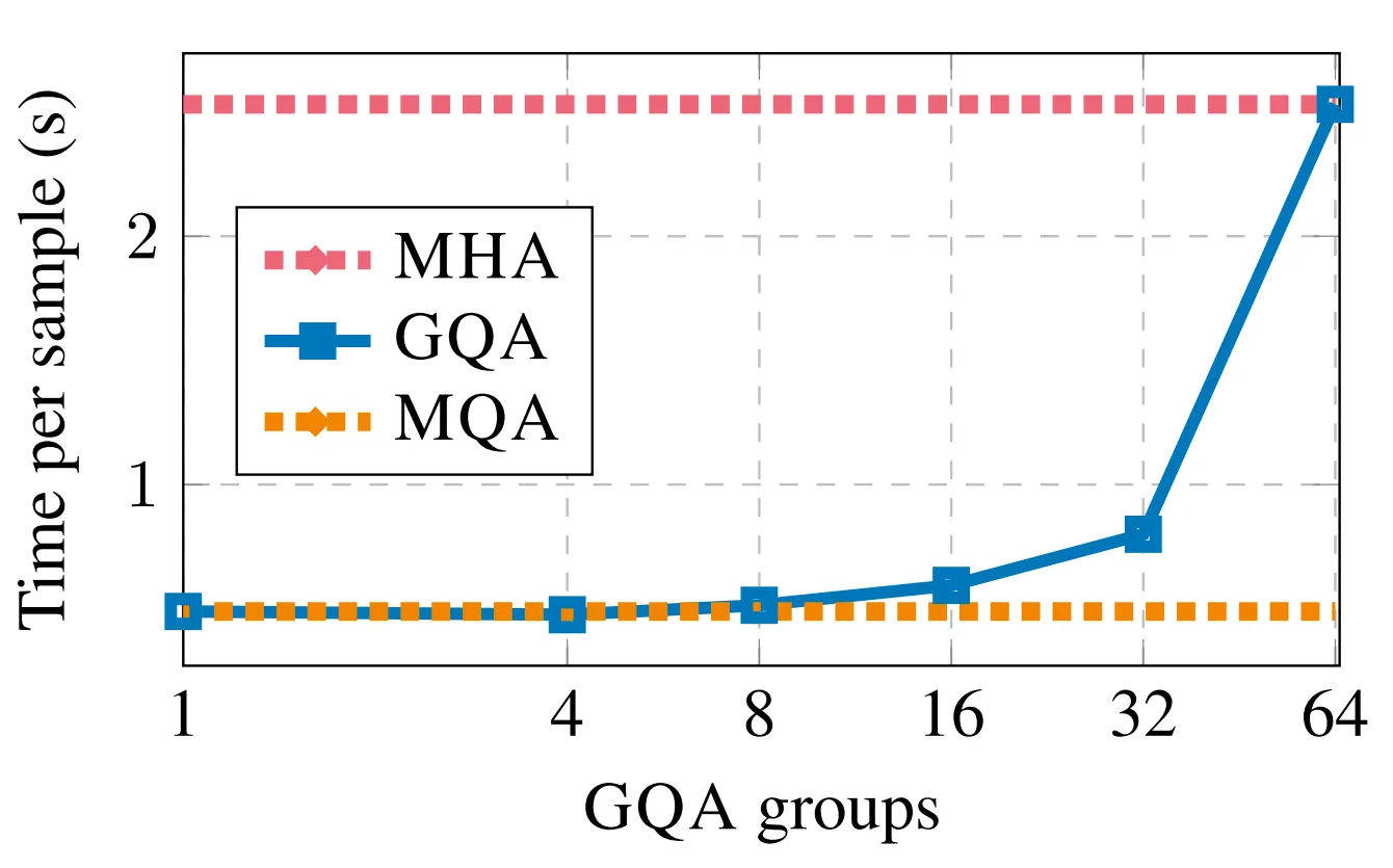
The result is a KV cache of around 550 MB per sequence—much larger than MQA’s 134 MB, but still a dramatic 8x reduction from MHA’s 4.3 GB.

Studies, including the original GQA paper, have shown that a well-trained GQA model can achieve nearly identical quality to its MHA counterpart while capturing most of the inference speed and memory benefits of MQA.

(I think this article is becoming too lengthy, but we’re getting to good places. Let’s continue…)

The Systems Hack: From FlashAttention to Its Sequels

Fixing the architecture with GQA solved the KV cache size problem. But another, more subtle bottleneck remained: the cost of memory access. Every step of the attention calculation (the matrix multiplies, the softmax, the dropout) required reading from and writing to the GPU’s main memory. This is where the physics of the hardware gets in the way.

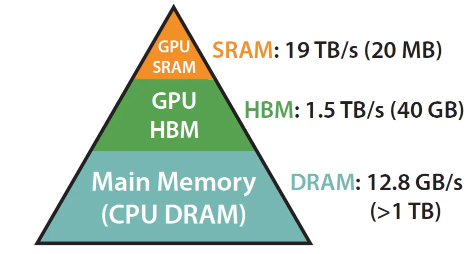
Think of your GPU’s large High-Bandwidth Memory (HBM) as a giant refrigerator and the tiny, lightning-fast SRAM on each compute core as your kitchen counter. A standard, naive implementation of attention is like cooking a recipe by taking one ingredient out of the fridge (HBM), doing one thing to it on the counter (SRAM), putting it back, and then getting the next ingredient. You spend more time walking back and forth to the fridge than you do actually cooking. The bottleneck isn’t the computation (the chopping); it’s the I/O.

This is the problem that FlashAttention, a brilliant innovation from researchers at Stanford (yes, viva Bay area…), set out to solve.

The core insight of FlashAttention is to be IO-aware. It redesigns the attention algorithm from the ground up to minimize those slow, expensive trips to HBM. It achieves this through two key techniques:

1. Kernel Fusion: Instead of launching separate GPU operations (kernels) for each step, FlashAttention fuses them into a single, monolithic kernel. This prevents the need to write massive intermediate results, like the full N x N attention matrix, back to HBM between steps.

2. Tiling: The algorithm breaks the large Q, K, and V matrices into smaller blocks, or “tiles,” that are small enough to fit into the fast on-chip SRAM. It then loads a block of Q and a block of K into SRAM, performs the full attention calculation for just that block, and only writes the final, much smaller output back to HBM. It iterates through the blocks, keeping the entire pipeline “hot” on the chip.

It’s like a master chef who gets all the ingredients for one stage of the recipe out onto the counter at once, does all the work there, and only puts the finished component back in the fridge.

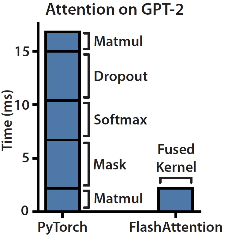
FlashAttention and its successors represent a different axis of optimization. While GQA changed the architecture to make the problem smaller, FlashAttention changed the implementation to solve the same problem more efficiently on the metal.

Outro

If you have got to this place means you enjoyed it. I won’t bother you more than I’ve already had. Wish you a good time till next week. TC.