Breaking the Quadratic Barrier

September 9, 2025 · #llm

In the last year, the goalposts for language models have shifted dramatically. We’ve gone from celebrating 32,000-token context windows to seeing demos of models that can ingest a million tokens in a single prompt—the entirety of War and Peace, an entire codebase, or hours of video transcripts.

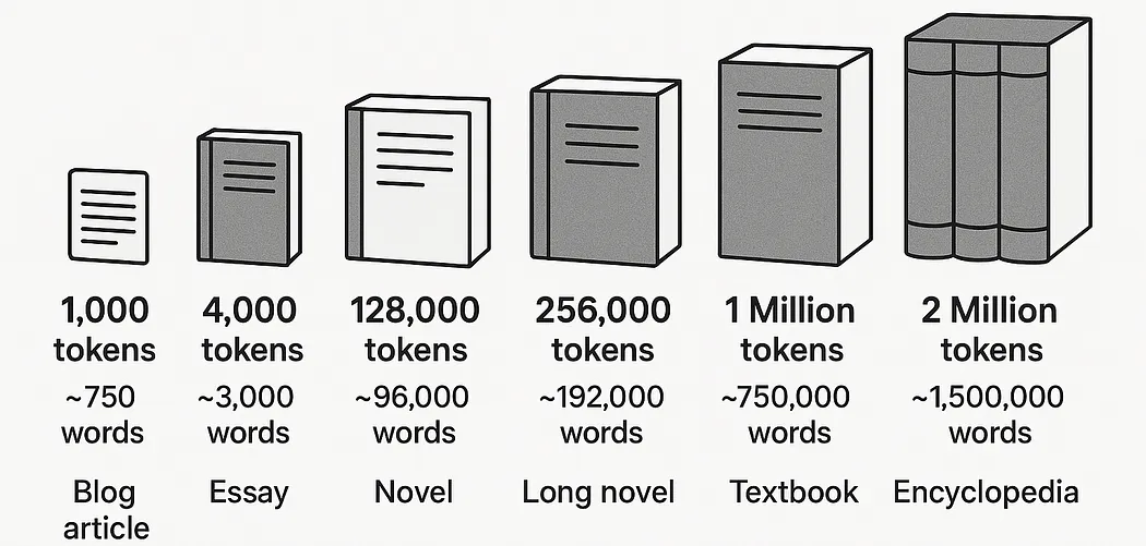
If you’ve been following along, this should feel… impossible.

In our previous discussions, we established that the computational and memory cost of self-attention is brutally expensive, scaling quadratically with the sequence length N. The complexity is O(N^2).

Let’s do the math for a one-million-token context window (N=1,000,000):

That’s a trillion elements in the attention matrix. Just storing that matrix, let alone computing it, would require terabytes of VRAM for a single layer of a single forward pass. Even with all the kernel-level magic of FlashAttention, the sheer number of floating-point operations would grind any current hardware to a halt.

So, how are these models doing it?

The short answer is: they’re not playing the same game. They are “cheating” the quadratic law. Instead of using dense, all-to-all attention, they use a toolbox of sophisticated sparse attention mechanisms. The core insight behind all these methods is that you don’t actually need every token to talk to every other token. A cleverly chosen, structured subset of connections is good enough.

In this deep dive, we’ll unpack the main families of these architectural hacks, from the simple neighborhood watch of Sliding Window Attention to the information-distilling power of Latent Attention. This is the story of how we broke the quadratic barrier.

Re-Confronting the Villain: The Unbreakable Quadratic Wall

In our last discussion, we celebrated the engineering hacks that made Transformer inference practical. Grouped-Query Attention (GQA) shrank the KV Cache, and FlashAttention optimized the low-level computation on the silicon. These are brilliant and essential optimizations, and they are the reason today’s models are as efficient as they are.

But they all share a limitation: they make the constant factor in our O(N^2) complexity smaller. They dramatically reduce the c in the c * N^2 cost function, but they can’t touch the exponent. They made the engine more efficient, but they didn’t change the fundamental laws of physics governing the system.

This isn’t an inconvenience; it’s a fundamental algorithmic barrier. You cannot brute-force your way through a quadratic wall at this scale. Improving the constant factor is a game of inches when what you need is a pole vault (that long stick that Olympics athletes use for jumping higher).

The only way out is to change the game. This has led to a new design philosophy built around a single concept: sparsity.

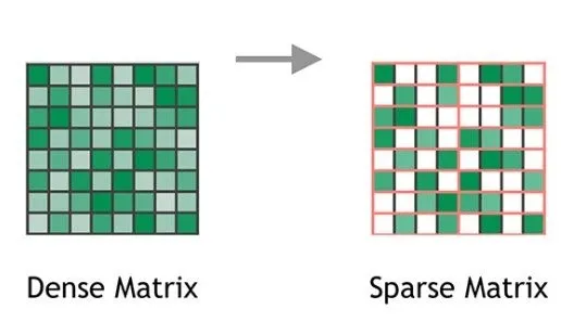
The core belief is that the dense N x N attention matrix is mostly redundant for any given token. The critical information for understanding a word’s meaning lies in a small, well-chosen subset of its peers. The rest is just noise. If you could intelligently ignore the vast majority of token-to-token connections, you could approximate the power of full attention without paying the crippling computational price.

This idea opened the floodgates for a whole new class of attention mechanisms, all trying to answer the same question: if we can only afford a few connections, which ones should we choose? Let’s start with the most intuitive answer.

The Neighborhood Watch - Sliding Window & Dilated Attention

If you can’t afford to have every token talk to every other token, the most logical first step is to have them talk to their immediate neighbors. This is the simple and powerful idea behind Sliding Window Attention.

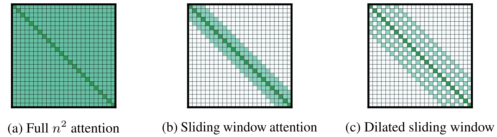
Instead of a full N x N attention matrix, each token is only allowed to attend to a fixed-size window of k tokens around it (e.g., k/2 tokens to the left and k/2 to the right). If your window size k is 4096, the 50,000th token in a sequence only looks at tokens 48,000 through 52,000, ignoring everything else.

The impact on complexity is exactly what we need. The computation is no longer dependent on the full sequence length N, but only on the fixed window size k.

Complexity changes from O(N^2) to O(N * k)=O(N)🥳.

Since k is a fixed hyperparameter (like 4096), the complexity is now effectively linear with respect to the sequence length N. Doubling the context from 100k to 200k tokens only doubles the compute, it doesn’t quadruple it. This technique, in its various forms, is the engine behind popular models like Mistral 7B.

The “Myopia” Problem

However, this efficiency comes at an obvious cost: the model becomes myopic. Important information can easily lie outside the local window. A character introduced in Chapter 1 of a novel might be crucial to understanding the plot twist in Chapter 50. With a simple sliding window, the model has no way to directly connect these two distant pieces of information. The information path is severed.

This is where a clever enhancement comes in: Dilated (or Strided) Sliding Windows (please check the image above).

To overcome myopia, we can give each attention head a different “view” of the context. While some heads might have a standard, dense sliding window, others can be configured with a “dilation factor.” A head with a dilation factor of d=2 would attend to every second token within its window. A head with d=4 would attend to every fourth token.

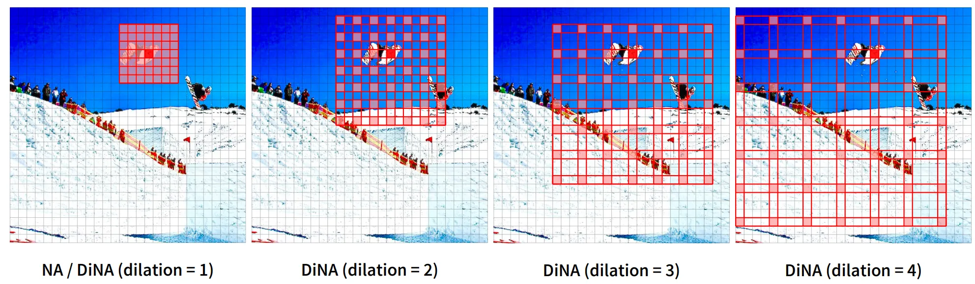
This is a brilliant trick. It allows the model’s “receptive field”, the total span of context it can theoretically access, to expand significantly without increasing the computational cost. By stacking layers with different dilation factors, information can “bubble up” from lower layers and travel across the entire sequence length, even if no single attention head ever sees the whole context at once.

Sliding Window Attention, especially when augmented with dilation, is the workhorse of modern long-context models. It’s simple, effective, and provides a robust baseline. But what if you knew, ahead of time, that some connections were more important than others?

Global and Structured Sparsity

Sliding windows, even with dilation, are still fundamentally “unintelligent.” They treat all tokens equally, assuming that proximity is the only thing that matters. But we know this isn’t true. In a long document or a complex codebase, some pieces of information are globally relevant, acting as anchors for the entire context.

This leads to a more structured approach, pioneered by influential models like Longformer and BigBird. Instead of just restricting attention, they augment it. The core idea is to combine the efficient local window with a few, pre-selected global connections.

Think of it as giving certain tokens a “VIP Pass”. While most tokens are stuck in their local neighborhood (the sliding window), a few special tokens are allowed to bypass this restriction and communicate across the entire sequence.

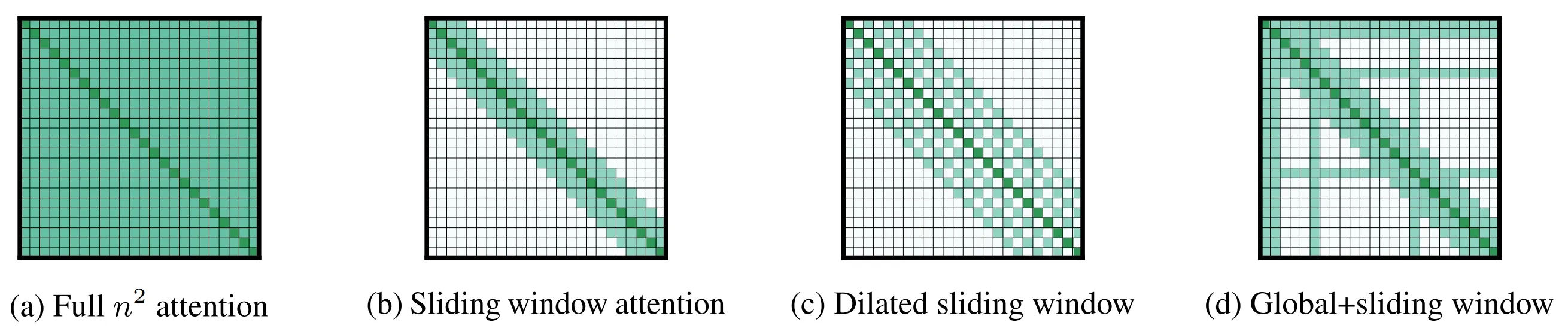
This is typically implemented as a combination of attention patterns within a single layer:

1. Local Window Attention: The majority of tokens still use the standard sliding window, efficiently capturing local context.

2. Global Attention: A small subset of pre-designated tokens can attend to every other token in the sequence, and crucially, every other token can attend back to them.

This analogy might help**:** Imagine a large city. Most daily interactions are local—you talk to your neighbors, shop at the local market (Sliding Window). But critical infrastructure like City Hall, the main hospital, or the central train station are accessible from everywhere, and they serve everyone (Global Tokens). These global nodes act as information highways, allowing a problem in one neighborhood to be communicated to the entire city.

So, who gets the VIP pass?
The choice of global tokens is critical. In BERT-style models fine-tuned for classification, the [CLS] token is a natural candidate. It’s designed to aggregate information from the entire sequence, so it makes sense to give it global access. For other tasks, the global tokens might be related to specific queries or concepts that are known to be important.

By combining these patterns, you get the best of both worlds: the O(N*k) efficiency of sliding windows for the bulk of the computation, plus the power of long-range dependencies for the information that truly matters. The added cost of the few global connections is minimal, but the increase in the model’s ability to reason over long documents is profound.

The Divide-and-Conquer - Hierarchical Attention

The previous methods—sliding windows and global tokens—still operate on a “flat” sequence of tokens. They simply prune connections within a single, massive attention matrix. But what if we could avoid building that massive matrix altogether by changing our perspective?

This is the central idea of Hierarchical Attention, a classic “divide and conquer” strategy. This approach has been explored in various forms, with a clear example being the architecture detailed in Google’s paper, “ETC: Extended Transformer Construction”.

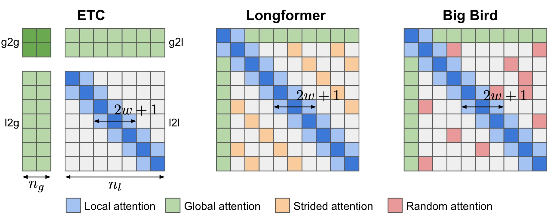
The process breaks the problem down into a multi-stage pyramid:

1. Divide: The full sequence of N tokens is first broken down into C smaller, non-overlapping chunks, each of length L. For example, a 100,000-token document could be divided into 200 chunks of 512 tokens each.

2. Conquer (Level 1 - Intra-Chunk): A standard attention mechanism is run independently over each of the C chunks. This is computationally cheap because L is small. The purpose of this stage is to “summarize” each chunk, often by extracting a single representative vector (like the output of a special [CLS] token for that chunk).

3. Conquer (Level 2 - Inter-Chunk): We now have C summary vectors, one for each chunk. A second level of attention is then performed only on this sequence of summary vectors. Since C is much smaller than the original N, this step is also very fast.

The analogy is how humans process long documents. You don’t keep every word of a book in your active memory. You read sentences to understand the meaning of a paragraph (Level 1), and then you mentally stitch together the high-level concepts from each paragraph to understand the argument of a chapter (Level 2).

The computational win is significant. Instead of one massive O(N^2) operation, we have many small O(L^2) operations and one O(C^2) operation. By choosing the chunk size appropriately, the overall complexity can be reduced to roughly O(N * sqrt(N)), a massive improvement.

This method’s trade-off is its structural assumption: it creates hard boundaries between chunks at the lowest level. Two closely related ideas that happen to fall on either side of a chunk boundary can’t interact directly. The model relies on the “summary” vectors to be good enough to preserve all the critical information, which can sometimes be a lossy compression.

The Hybrid Compressor - DeepSeek’s Multi-Head Latent Attention

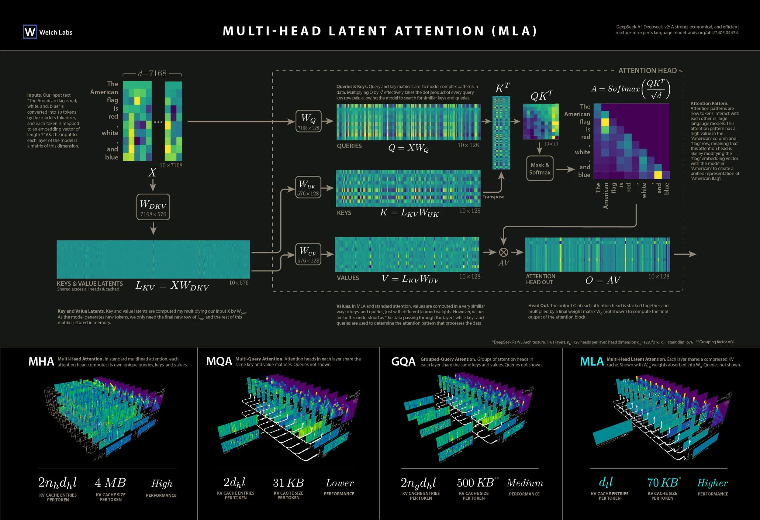
The previous hacks present different philosophical approaches to sparsity. But what does a state-of-the-art, production-ready implementation look like? The answer is often a clever combination of these ideas. A brilliant example of this is the Multi-head Latent Attention (MLA) mechanism introduced in the DeepSeek-V2 model.

Their approach isn’t a single technique but a hybrid attention system designed to achieve extreme efficiency during auto-regressive generation. It explicitly combines a local attention mechanism with a novel form of compressed global attention.

Here’s how it works:

1. High-Fidelity Local Context via Sliding Windows:
First, the model uses a standard Sliding Window Attention (SWA). For any new token being generated, it pays full, detailed attention to its most recent neighbors (e.g., the last 4,096 tokens). This ensures that the model has a perfect, high-fidelity view of the immediate local context, which is critical for grammatical correctness and coherence.

2. Compressed Global Context via Latent Attention:
This is the core innovation. For the vast history of tokens that lie before the sliding window, DeepSeek doesn’t store the full KV cache. Doing so would create the memory bomb we’re trying to avoid. Instead, it uses a learned projection to actively compress the distant KV cache into a small, fixed-size set of “latent” KV pairs.

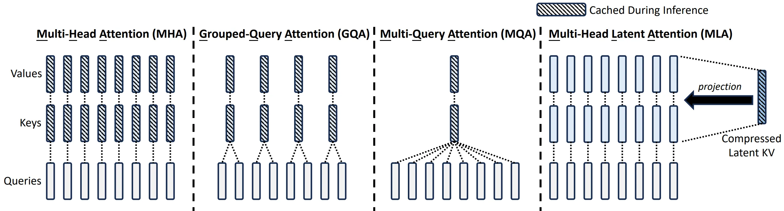
The Analogy: Imagine you’re reading a very long book.

• Sliding Window: You keep the last 10 pages you just read spread out on your desk in full detail.

• Latent Compression: For the first 500 pages of the book, you don’t keep all 500 pages. Instead, you maintain a single page of summary notes (“latent KVs”) that captures the key characters, plot points, and themes. As you read, you keep updating this summary page.

When the model generates a new token, its Query vector attends to two sources of information simultaneously:

1. The full, detailed KV pairs from the recent sliding window.

2. The small, compressed set of latent KV pairs that represent the entire distant past.

The engineering benefits are massive. The size of the KV cache is no longer dependent on the total sequence length N. It’s dependent only on the size of the local window (k) and the size of the compressed latent set (m), both of which are small, fixed constants.

• Complexity is O(N * (k + m)), which is linear.

• KV Cache Memory is dramatically reduced, allowing for huge context windows (like DeepSeek’s 128k) and high-throughput batching.

Outro

Like always, I thank you have read so far. I think this is going to be the last article about attention for a while as we have covered a lot of ground on this topic with this and the last 2 article. I don’t know any other attention mechanism currently in production that is out of these variants introduced. Will keep these articles updated though.

With that, wish you great week ahead.