RoPE: The Phase Geometry Behind Long-Context Transformers

June 6, 2026 · #llm#llm#positional embedding#rope

I’ve been absent for a relatively long time (6 months). I was working on my mathematical base and deepening my knowledge of language models (and recently diffusion models). Today I was working on implementing RoPE (checkout the paper) in numpy (code at the end of the article), and stumbled upon a visualization that was so amazing I couldn’t pass on not sharing it. Without any more fluff, let me share it.

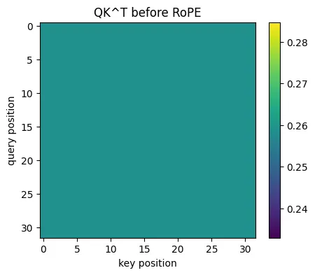
The following shows attention score before applying rope. Interpretation is that all tokens uniformly attend to all others.

But look at what happens after RoPE. There is no uniformity. Each token as pockets of attention.

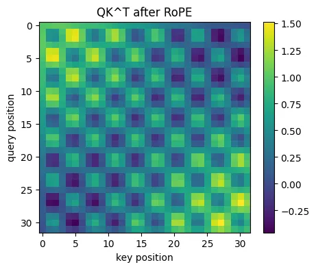
The pockets that are lighter are where positional encoding aligns better.

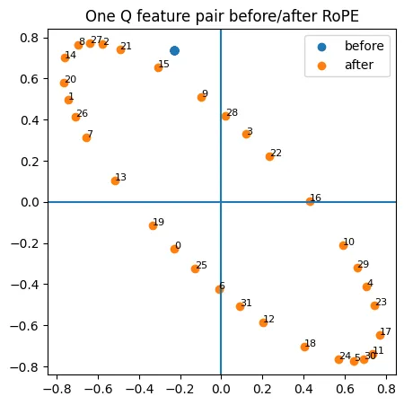
Now let’s go to the next visualization. This shows how the first dimension across different tokens are encoded. Can you see the circular or rotary encoding of the tokens? Hint: can you follow from token 1 → N? Isn’t this amazing? this is visualization of what they named it Rotary Positional Embedding (RoPE).

This is another visualization, for the 2nd dimension pair, across tokens:

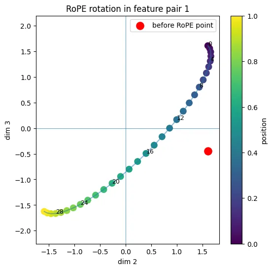
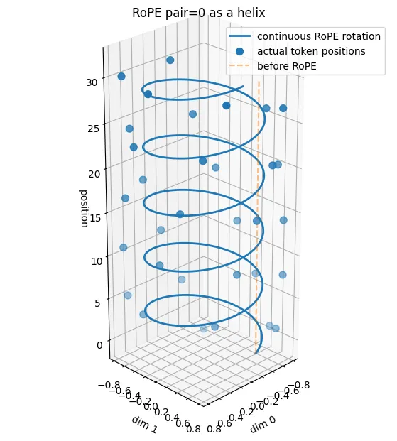
And this is the 3d visualization across time (position):

In case you’d love to play with it, here is my code:

import numpy as np

def apply_rope(k, q, base = 10_000):
    eps = 1e-6
    D = k.shape[-1]
    T = k.shape[-2]
    # theta = base ^ (-2m/d)
    # print(m/(np.arange(0,m,2)+eps))
    theta = base ** (-2 * np.arange(D // 2) / D)
    pos = np.arange(T)
    angle = pos[:, None] * theta[None, :]

    print(theta)
    print(angle.shape)
    
    cos = np.cos(angle)
    sin = np.sin(angle)

    def apply_single(x):
        out = np.empty_like(x)
        x_even = x[:,:,::2]
        x_odd = x[:,:,1::2]

        out[:,:,::2] = cos * x_even - sin * x_odd
        out[:,:,1::2] = cos * x_even + sin * x_odd

        return out
    return apply_single(k), apply_single(q)

import numpy as np
import matplotlib.pyplot as plt

B = 1
T = 32
D = 8

# Same content at every position
base_q = np.random.randn(D)
base_k = np.random.randn(D)

Q = np.tile(base_q, (B, T, 1))
K = np.tile(base_k, (B, T, 1))

K_rope, Q_rope = apply_rope(K, Q)

def attn_scores(Q, K):
    return Q[0] @ K[0].T / np.sqrt(Q.shape[-1])

S_before = attn_scores(Q, K)
S_after = attn_scores(Q_rope, K_rope)

plt.figure(figsize=(5, 4))
plt.imshow(S_after)
plt.title("QK^T after RoPE")
plt.xlabel("key position")
plt.ylabel("query position")
plt.colorbar()
plt.show()

# Show rotation in 2D
pair = 0
a = 2 * pair
b = 2 * pair + 1

plt.figure(figsize=(5, 5))
plt.scatter(Q[0, :, a], Q[0, :, b], label="before")
plt.scatter(Q_rope[0, :, a], Q_rope[0, :, b], label="after")

for t in range(T):
    plt.text(Q_rope[0, t, a], Q_rope[0, t, b], str(t), fontsize=8)

plt.axhline(0)
plt.axvline(0)
plt.axis("equal")
plt.title("One Q feature pair before/after RoPE")
plt.legend()
plt.show()