How MoE Powers Modern LLMs

August 6, 2025 · #llm

When DeepSeek-V2 released their model, it caught a lot of attention—not just because it was big, but because it was efficient. The model had over 200 billion parameters, yet it managed to be faster and cheaper to run than smaller dense models. They pulled that off using Mixture of Experts (MoE).

MoE isn’t some brand-new idea. Google explored it a few years ago with GShard and Switch Transformer, but DeepSeek’s implementation made it clear that this architecture is ready for real-world use. It even made waves outside the ML world and caused 17% Nvidia stock crash on 27 Jan 2025, mostly due to speculation that MoE models might reduce GPU demand. That turned out to be some over reaction. If anything, MoE just makes GPUs more efficient. And to be honest with you, I think we are far from our target scale or maturity that would bring down GPU demand. We can have a coffee about this and chat ;).

At its core, MoE is pretty simple. Instead of running every part of the model for every token, you only run a few specialized parts—experts—based on what’s needed. This allows the model to scale in parameter count without scaling compute and memory costs the same way.

In this post, I’ll break down how MoE works, why it matters, and how it’s being used in modern LLMs. If you’re curious about scaling strategies, system performance, or just want to understand what’s happening inside models like DeepSeek or Switch Transformer, this should give you a solid picture without getting too theoretical.

The Scaling Wall of Dense Models

For years, the formula for better AI models was simple: make them bigger. Research, particularly from papers like Google’s “Chinchilla”(Training Compute-Optimal Large Language Models), established a clear trend known as scaling laws. These laws show that as you increase a model’s parameter count and train it on more data, its performance reliably improves. This led to an arms race to build ever-larger dense models, where every parameter is used to process every single token of input.

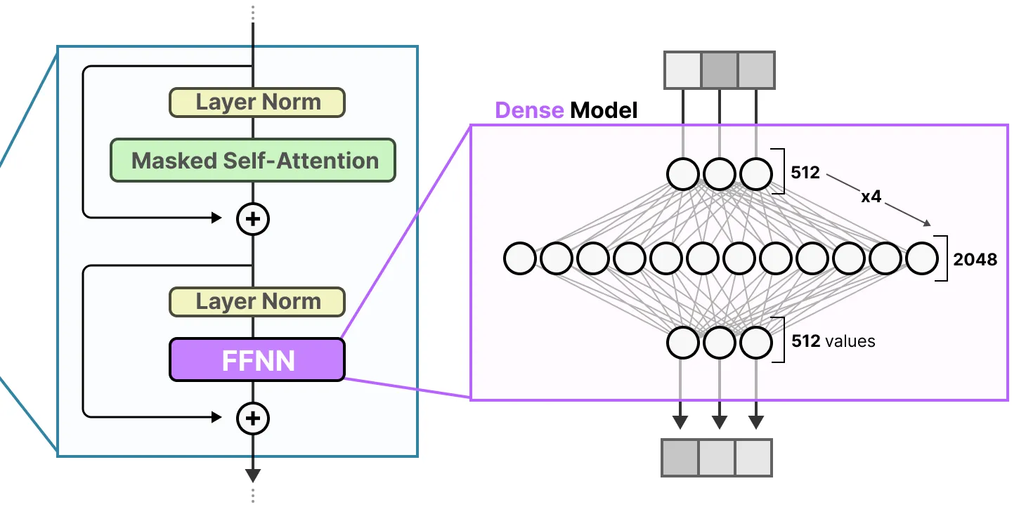
But this approach comes with a punishing trade-off. The cost of running these models doesn’t just grow—it skyrockets. For a dense model, the computational cost (measured in Floating Point Operations, or FLOPs) is directly proportional to its parameter count.

This creates two major bottlenecks:

1. Crippling Inference Costs: Every user query requires activating the entire multi-billion parameter network. This translates to high energy consumption, a need for more powerful (and expensive) GPUs, and slower response times (inference latency). At a certain scale, serving the model to millions of users becomes economically unfeasible.

2. Astronomical Training Demands: Training a state-of-the-art dense model can cost hundreds of millions of dollars and consume immense computational resources for weeks or months. This puts frontier AI development out of reach for everyone except a handful of hyperscale companies.

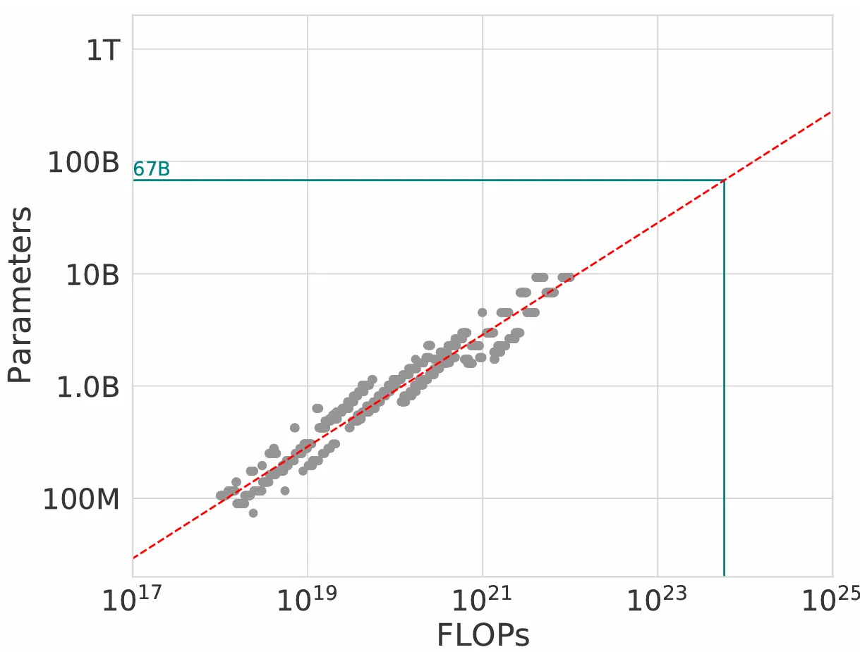
This is the scaling wall: we know that more parameters can lead to smarter models, but we’re hitting a hard physical and financial limit on how big we can practically make them. How can we get the benefits of a massive parameter count without the crippling computational cost?

You might ask why Chinese model used MoE first? Because they were hitting this scaling wall earlier than US-based firms. Instead of having access to cutting edge H100 NVidia cheaps, they just have H800 that is 20% less performant. So they needed to find a way around this.

💡 Case Study: Hitting the Wall Sooner

The scaling wall isn’t a theoretical problem that affects everyone at the same time—some hit it earlier than others. This is a key reason why Chinese firms were among the first to successfully deploy large-scale MoE models.

While US-based firms had access to NVIDIA’s top-tier H100 GPUs, export controls meant Chinese companies were limited to the H800, a chip with significantly less performance. They were forced to confront the limits of scaling with less powerful tools.

This hardware disadvantage created immense pressure to innovate on architecture. MoE wasn’t just an interesting experiment for them; it was a necessary strategy to stay competitive—a solution born from hitting a hard performance ceiling well before their rivals. Necessity, in this case, was the mother of architectural invention.

Enter the Mixture of Experts: The Specialist Committee in the Machine

If dense models are hitting a scaling wall, Mixture of Experts (MoE) is the architectural parkour that finds a way over it. It’s not about brute force; it’s about working smarter. At its heart, MoE reframes the problem: instead of asking one giant network to know everything, what if we could ask a small group of specialists instead?

The Core Analogy: The Specialist Committee

Imagine you’re building an ultimate question-answering machine.

The dense model approach is like hiring one single, superhuman generalist. This person has read every book, studied every field, and learned every language. To answer any question—whether it’s about quantum physics, Shakespearean sonnets, or a bug in a C++ program—they have to activate their entire brain. It’s incredibly powerful, but also incredibly slow and energy-intensive for every single task.

The MoE approach is like assembling a committee of world-class experts. You have a physicist, a poet, a historian, and a master programmer, each a genius in their own domain. When a question arrives, you don’t bother the whole committee. Instead, you have a clever front-desk receptionist—the “Router”—who instantly identifies the nature of the question.

“Ah, this one’s about linked lists,” the router says, and promptly directs the query to the programmer and perhaps the logician. The other experts—the physicist, the poet—get to sit this one out, saving their energy. The two chosen experts solve the problem, and the router combines their outputs into a single, polished answer.

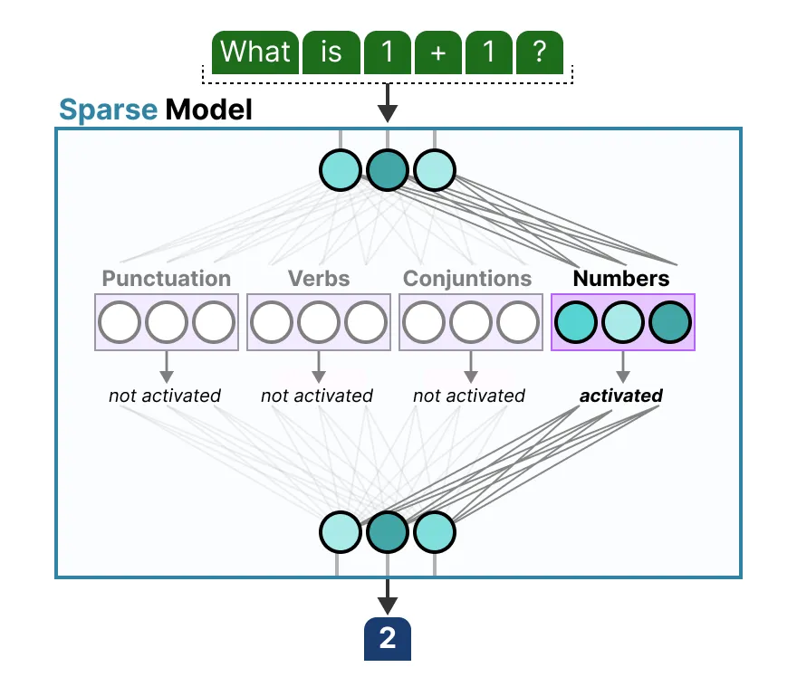
This is the genius of MoE: you get the collective knowledge of the entire committee (total parameters), but for any given task, you only pay the computational cost of consulting a few of them (active parameters).

Popping the Hood: The Two Key Components

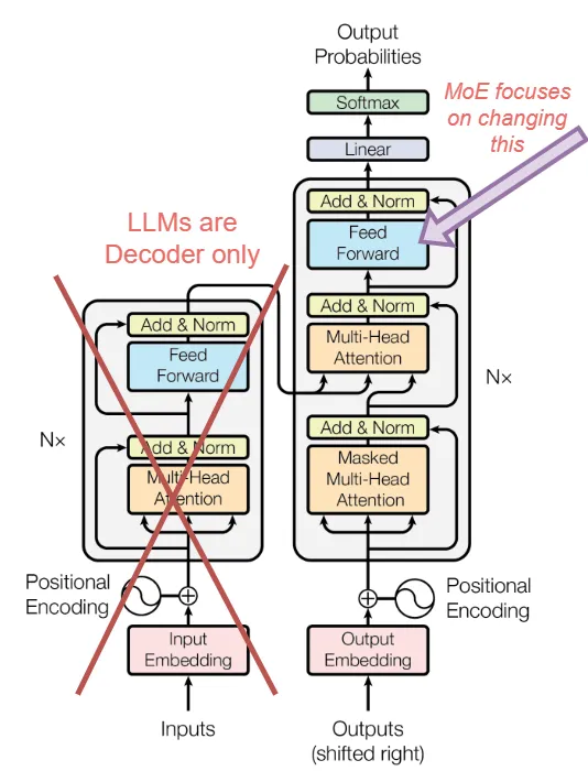
Let’s translate this analogy into silicon. In a Transformer, an MoE layer is designed to replace the standard Feed-Forward Network (FFN), which is one of the two major sub-layers in every block. Here’s how it’s built:

1. The Experts (The Committee Members)

These aren’t mysterious entities; they are simply standard neural networks. Specifically, each “expert” is a Feed-Forward Network, architecturally identical to the one it’s replacing. You might have 8, 16, or even 64 of these experts sitting side-by-side in a single MoE layer.

During training, these experts naturally begin to specialize. While not a perfect division, one expert might become adept at processing syntax in natural language, another at recognizing patterns in Python code, and a third at handling factual knowledge. They become a pool of specialized computational resources.

2. The Gating Network (The Router)

This is the brains of the operation. The gating network, or “router,” is a small, very fast neural network. Its one and only job is to play matchmaker between incoming tokens and the pool of experts.

For every single token that arrives at the layer, the router looks at it and generates a set of scores—one for each expert. These scores represent the router’s confidence that a given expert is the right one for the job.

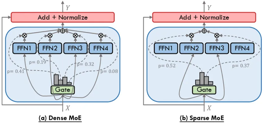
We have 2 flavours of MoE: Dense and Sparse MoE. In the Dense MoE version all experts are activated to the proportion of their weight. But the crucial trick for Sparse MoE is: instead of using all the experts in proportion to their scores (which would be inefficient), the router employs Top-K Gating. It simply picks the experts with the k highest scores and sends the token only to them. For most modern LLMs like Mixtral and DBRX, k is a very small number, typically 2 or 4.

The final output for the token is then a weighted sum of the outputs from just these top k experts, with the weights determined by their original scores from the router. It’s like a carefully blended cocktail of specialist opinions.

This architectural switch is the magic trick behind models like DeepSeek-V2. By having a vast library of 236 billion parameters but only reading 21 billion of them for any given token, they achieve the knowledge capacity of a huge model with the speed and cost of a much smaller one.

This simple but powerful idea has profound consequences for model performance and efficiency, which fundamentally changes the economics of training and serving billion-scale models.

Activation Params and the Math of Efficiency

The magic of Mixture of Experts isn’t just a conceptual trick; it’s a mathematical advantage rooted in how computation is performed. By moving from a dense to a sparse architecture, MoE fundamentally changes the relationship between a model’s size and its operational cost. Let’s break down the numbers.

The Cost of Being Dense

In a standard Transformer, the Feed-Forward Network (FFN) layers are the most computationally expensive part, far more so than the attention mechanism. The computational cost (FLOPs) of an FFN layer is roughly proportional to twice its parameter count, as each token’s vector is multiplied by two weight matrices.

For a dense model, the math is straightforward. The active parameters are the total parameters.

Where Pffn is the number of parameters in that FFN layer. If you want to double the “knowledge” of your model by doubling the parameters in its FFNs, you also double the computational work required to process every single token. This linear scaling is the unforgiving math that leads directly to the scaling wall.

The Efficiency Math of MoE

Now, let’s introduce the MoE layer. Instead of one large FFN, we have a collection of N smaller “expert” FFNs. For any given token, the router selects the top k experts.

The parameters in an MoE layer are split into two categories:

Total Parameters (Ptotal): This is the full knowledge base of the layer. It’s the number of experts multiplied by the parameters per expert.

(We can ignore the tiny router’s parameter count for this calculation.)

Active Parameters (Pactive): This is the number of parameters that are actually used to process a single token. This is the k chosen experts multiplied by the parameters per expert.

This distinction is everything. The computational cost is determined by the active parameters, not the total.

Hold on—did we just solve a multi-billion dollar scaling problem with some simple multiplication? Pretty much! This is the beautiful math that lets MoE break the rules. Before we see it in action, let that core idea sink in: we get the knowledge of all the experts, but only pay the price for a few.

A Concrete Example: Mixtral 8x7B

Let’s see this in action with the celebrated Mixtral 8x7B model. Its name gives us the key variables: it has N=8 experts, and it’s built on a 7B parameter base architecture. Its router selects k=2 experts per token.

_💡_The Rule of Thumb for MoE Naming

So, here is the rule of thumb you can use for understanding models like Mixtral or Databricks’ DBRX Instruct (which uses a similar naming scheme):

The Y in a model named NxYB refers to the approximate size class of the base dense model from which it was constructed. It’s a way of communicating that the model’s core, non-expert components (like attention) are similar in size and complexity to those found in a well-understood Y-billion parameter dense model. The real parameter breakdown requires looking at the shared vs. expert parameter counts, which are now clearly established for Mixtral.

Let’s focus on the FFN layers:

A single expert’s FFN size (Pexpert):

Let’s calculate the size of one expert across all 32 layers:

Pexpert = num_hidden_layers × (P_gate + P_up + P_down)
Pexpert = 32 × (4096 × 14336 + 4096 × 14336 + 14336 × 4096)
Pexpert = 32 × (58,720,256 + 58,720,256 + 58,720,256)
Pexpert = 32 × (176,160,768)
Pexpert ≈ 5.64 Billion

Total FFN Parameters (Ptotal): 8 experts × 5.64B ≈ 45.12B. This is the true size of Mixtral’s knowledge in its MoE layers.

Active FFN Parameters (Pactive): 2 experts × 5.64B = 11.28B. This is the amount of compute it actually performs. This pretty much maps out to what Mistral published in their news release.

Now, compare the computational load:

• Mixtral’s FLOPs: Proportional to its 12.9B(11.28B experts + 1.6B shared blocks like attention and embeddings) active FFN parameters.

• A dense model’s FLOPs (with similar knowledge): A dense model with a comparable 45.12B FFN would have its FLOPs proportional to all ~46.7B (45.12B FFN + 1.6B shared blocks like attention and embeddings**)**parameters.

By dividing the two, we see the efficiency gain:

The Mixtral model performs 3.6 times less computation in its MoE layers than a dense model of equivalent knowledge capacity. It effectively operates with the speed and cost of a ~13B dense model (1.6B non-FFN params + 11.28B active FFN params, roughly) while leveraging the representational power of a ~47B model.

This is the mathematical foundation of MoE’s success. It isn’t a free lunch—it introduces new engineering challenges we’ll discuss next—but it provides a powerful recipe for building larger, more knowledgeable models without the crippling computational price tag.

No Free Lunch: The Challenges and Trade-offs of MoE

The promise of Mixture of Experts is spectacular, but implementing it at scale is a masterclass in system design and trade-offs. MoE cleverly dodges the dense model’s compute problem but, in doing so, creates new and complex challenges in memory, network communication, and training stability.

Challenge 1: The Massive Memory (VRAM) Footprint

This is the most significant trade-off. While computation is sparse (only k experts are active), memory is dense. All parameters for all experts must be loaded into the GPU’s high-bandwidth memory (VRAM) at all times.

Think back to our specialist committee analogy: you only talk to a few experts at a time, but the entire committee must be present in the building, ready to be called upon.

For a model like Mixtral 46.7B, this means finding enough VRAM across a cluster of GPUs to hold all 46.7 billion parameters, even though you only use 12.9 billion for any given token. This immediately makes running large MoE models impossible on consumer hardware and requires sophisticated, multi-GPU servers. MoE essentially trades a compute-bound problem for a memory-bound problem.

The standard solution is Expert Parallelism, where the model is partitioned across multiple GPUs. Instead of trying to fit the whole model on one device, you place different experts on different GPUs. For example, in an 8-expert model running on 8 GPUs, each GPU might hold one expert. This solves the memory issue, but it directly creates the next challenge.

Challenge 2: The All-to-All Communication Bottleneck

Once you’ve spread your experts across different GPUs, you create a new problem: network overhead. The gating network on GPU 1 might decide a token needs to be processed by Expert #5, which lives on GPU 5. That token’s data must now be sent across the network from GPU 1 to GPU 5.

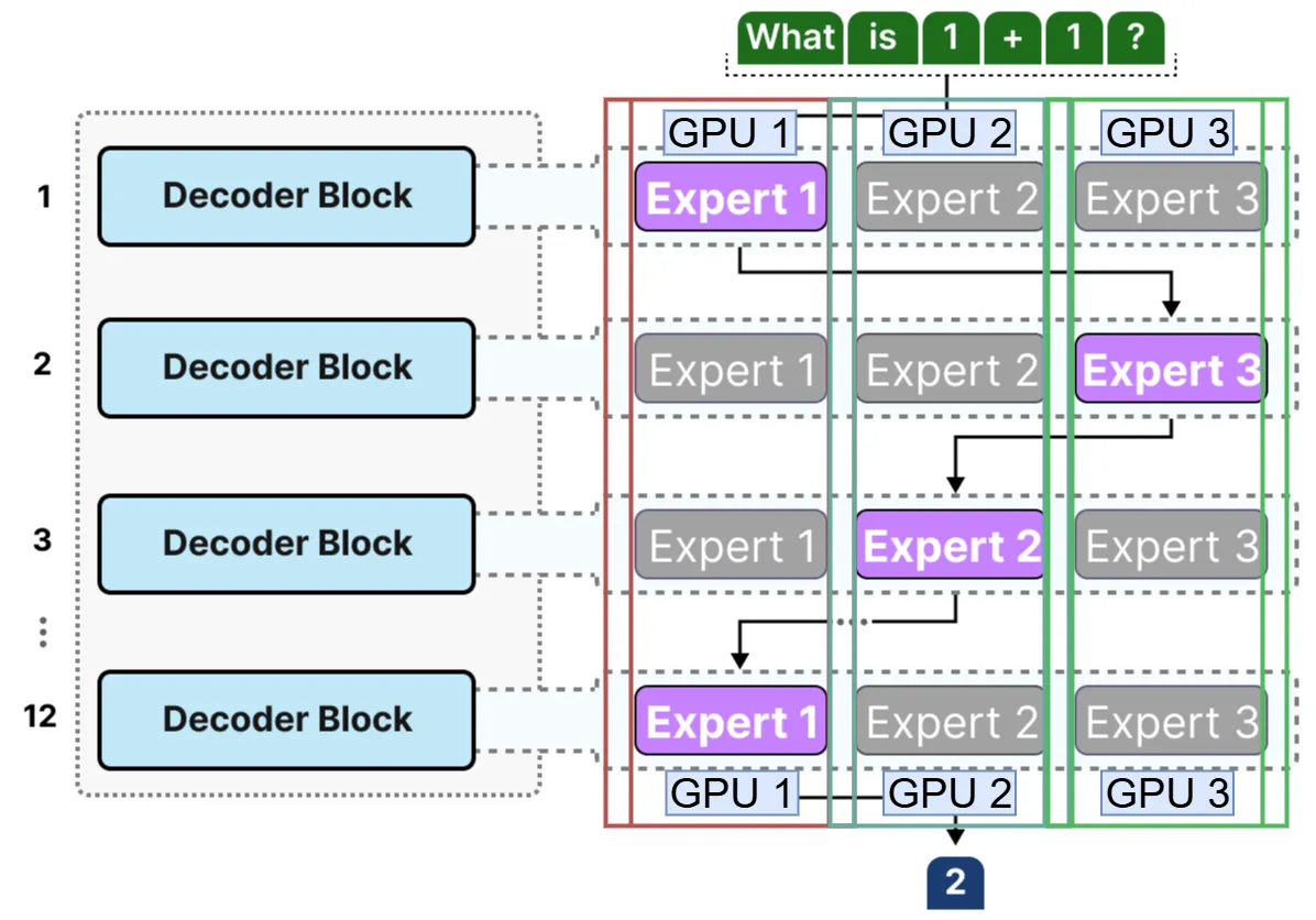
This requires a bandwidth-intensive communication step called an All-to-All operation.

Imagine a busy post office. A batch of tokens (letters) arrives at each GPU (clerk). The router on that GPU sorts the tokens based on which expert (destination city) they need to go to. Then, all GPUs must perform a massive, synchronized exchange, sending and receiving tokens to and from every other GPU in the cluster. After the experts do their work, the results must be shuffled back to their original GPUs.

This All-to-All shuffle is pure communication overhead. It doesn’t perform any useful computation and can become a major bottleneck if the network interconnect between GPUs (like NVLink or InfiniBand) is not fast enough. This challenge, extensively analyzed in Google’s GShard paper, is often the single biggest factor limiting the scalability of MoE training.

Challenge 3: Load Balancing and “Lazy” Routers

This is the key algorithmic challenge. The gating network is a neural network, and its goal is to minimize loss. What happens if it discovers that Expert #3 is particularly good at processing the most common types of tokens in the training data?

It might get lazy and develop a “favorite,” sending a disproportionate number of tokens to that expert. This leads to two disastrous outcomes:

1. Expert Starvation: Other experts receive very few tokens, remain under-trained, and their parameters are essentially wasted.

2. Computational Bottleneck: The GPU holding the “favorite” expert is constantly overworked, while the other GPUs sit idle, waiting for it to finish.

To combat this, MoE models add an Auxiliary Load Balancing Loss to the main training objective. This loss function is designed to incentivize the router to distribute tokens as evenly as possible across all available experts. As formalized in the Switch Transformer paper, it adds a small penalty if either the number of tokens sent to each expert or the router’s probability scores for each expert become too imbalanced.

Finding the right weight for this auxiliary loss is a critical and delicate part of training a stable, high-performing MoE model.

Architectural Evolution: The Shared Expert

The challenges of load balancing and expert specialization aren’t just theoretical; they are active areas of architectural innovation. As it turns out, forcing every expert to learn everything from scratch—from basic syntax to specialized knowledge—is inefficient. This has led to one of the most elegant recent evolutions in MoE design: the introduction of a shared expert.

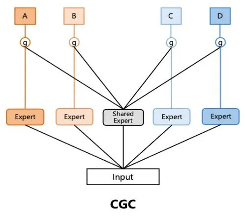
This advanced pattern, notably used in models like DeepSeek-V2, modifies the standard MoE layer by splitting the “expert” workload into two distinct types.

1. Routed Experts: These are the specialists in our committee. There are N of them, and the router selects the top-k for each token to handle specialized processing.

2. Shared Expert: This is a single, dense FFN layer that every token passes through, regardless of the router’s decision. It operates in parallel to the specialists.

The “Chief of Staff” Analogy

To update our committee analogy, think of the shared expert as a highly competent Chief of Staff.

Every request first goes to the Chief of Staff. They handle all the foundational, universal tasks—clarifying language, attaching common facts, and standardizing the format. Only after this pre-processing does the router get the request. The router’s job is now vastly simpler; it can focus on matching the core essence of the query to the true specialists (the routed experts). The final answer combines the foundational work of the Chief of Staff with the deep insights from the chosen specialists.

The Technical Payoff

This design isn’t just more elegant; it’s a direct solution to key MoE challenges:

• Factoring Out Common Knowledge: The shared expert learns the common patterns present in all language (syntax, grammar, basic semantics). This frees the routed experts from wasting their limited capacity on re-learning these universal concepts, allowing them to become more deeply specialized in their unique domains.

• Improved Routing and Specialization: By offloading the “easy” work to the shared expert, the router can make more meaningful decisions based on a token’s core semantic content. This leads to more effective specialization and better load distribution, as the router isn’t just defaulting to a few “generalist” experts.

• Enhanced Stability: The shared expert provides a consistent computational path and gradient flow for every token in the sequence, which contributes to more stable and reliable training.

This architectural pattern shows that the future of MoE isn’t just about adding more experts, but about creating more sophisticated and collaborative relationships between them. It’s a move from a simple committee to a highly organized and efficient team.

MoE in the Wild: The Models Leading the Charge

The journey of MoE from a promising research concept to a production-ready powerhouse has been marked by a few landmark models. Each one solved a key problem or demonstrated a new level of scale, paving the way for the next.

The Pioneers: Google’s GShard and Switch Transformer

Long before MoE entered the mainstream consciousness, Google Brain was laying the groundwork.

• GShard (2020): This was the model that proved MoE could work in the demanding, real-world environment of Google Translate. The GShard paper (Lepikhin et al., 2020) was foundational, demonstrating how to scale a Transformer to 600 billion parameters. Crucially, it introduced expert parallelism as the canonical solution to the memory problem and detailed the system design required to handle the All-to-All communication bottleneck across hundreds of TPU devices.

• Switch Transformer (2021): If GShard was the engineering proof, Switch Transformer was the scaling statement. In their paper (Fedus et al., 2021), the Google team pushed the architecture to an astonishing 1.6 trillion parameters (Switch-C). They simplified the routing algorithm to top-1 and rigorously studied the auxiliary load balancing loss needed to prevent expert starvation, making large-scale training more stable.

The Open-Source Wave: Mixtral and DBRX

These are the models that brought MoE out of the hyperscale data centers and into the hands of the broader developer community, proving their practical value.

• Mixtral 8x7B (Mistral AI): The model that changed the game for open-source AI. By using a top-2 router with 8 experts, Mixtral delivered performance that matched or beat much larger dense models like Llama 2 70B, but with 6x faster inference. Its architecture (sharing attention parameters while “expert-ifying” the FFNs) provided a brilliant template for cost-performance trade-offs.

• DBRX (Databricks): Following Mixtral’s success, DBRX demonstrated a different design philosophy. Instead of a few large experts, it opted for a more “fine-grained” approach with 16 smaller experts, of which it activates k=4. This showcased that there isn’t one single “right” way to build an MoE.

The Mainstream Titan: Meta’s Llama 4

Meta’s entry into the MoE space solidified the architecture as the de facto standard for frontier open models. The release of the Llama 4 “herd” in April 2025 was a clear signal that the era of large dense models was over, replaced by a new paradigm of sparse, specialized architectures.

Instead of a single model, Meta released a family of MoE models showcasing two distinct and sophisticated design philosophies:

• Llama 4 Maverick (~400B total): Designed for peak performance, Maverick features an astonishing 128 experts. It employs an advanced alternating architecture, where standard dense Transformer layers are interspersed with MoE layers. In these MoE layers, it uses a highly efficient routing strategy that combines one shared expert with just one (k=1) routed expert per token. This fine-grained specialization allows it to access its vast knowledge base with surgical precision.

• Llama 4 Scout (~109B total): Optimized for maximum efficiency and a massive context window, Scout uses a more conventional full MoE architecture with 16 experts. This design choice focuses on delivering robust performance across a wide range of tasks while being more straightforward to deploy and manage.

Remarkably, despite their different total parameter counts and internal designs, both models feature a consistent 17B active parameters. This demonstrates a mature strategy of offering varied knowledge capacities at a fixed computational cost. The native multimodality of the Llama 4 family, integrating text and image processing from the ground up, combined with its wholehearted adoption of advanced MoE principles, served as the ultimate validation of the architecture for building the next generation of AI.

The Efficiency Frontier: DeepSeek-V2

Circling back to the model that inspired this article, DeepSeek-V2 represents the cutting edge of MoE efficiency.

• DeepSeek-V2 (2024): DeepSeek AI took the core MoE concept and evolved it. Their 236B parameter model only activates 21B parameters per token—an incredible 11:1 ratio of total-to-active parameters. They achieved this by innovating on the architecture itself, introducing MLA (Multi-head Latent Attention), which allows for sharing experts not just in the FFN layers but also within the attention mechanism itself. This further reduces the active parameter count and inference cost, setting a new standard for what is possible in terms of sparse model efficiency.

The Future is Sparse and Specialized

For years, the path to more capable AI seemed to be a one-way street paved with ever-denser, ever-larger models—a path leading directly to a computational and financial wall. The Mixture of Experts architecture hasn’t just offered a detour; it has redrawn the map entirely.

We’ve seen that MoE is not magic, but a sophisticated engineering trade-off. It brilliantly sidesteps the crippling FLOPs cost of dense models by swapping a compute-bound problem for a memory-and-network-bound one. By activating only a fraction of its vast parameter count for any given token, an MoE model delivers the knowledge capacity of a giant with the operational cost of a much smaller counterpart. This is the principle that allows Mixtral to outperform a larger dense model at 6x the speed and enables DeepSeek-V2 to achieve its incredible efficiency.

The success of MoE, crowned by its adoption in mainstream models like Meta’s Llama 4, marks a fundamental paradigm shift. We are moving away from an era defined by scaling through brute-force density and toward one that values architectural intelligence. The goal is no longer just to build bigger models, but to build smarter, more efficient systems that maximize their capacity while minimizing their cost.

At the end, I hope you enjoyed reading this article as much as I enjoyed researching and writing it.